Annex "Fish"
Annex 1. Short description of the selected monitoring programmes
The selected fish monitoring programmes covered a time span of at least 10 years, up to the present. This annex presents a short description of the methods of these monitoring programmes. A comprehensive overview of all fish monitoring activity is being prepared by the CWSS TMAP fish monitoring subgroup (pers. com. A. Dänhardt).
DFS beam trawl
The Dutch Demersal Fish Survey (DFS) covers coastal waters (up to 25 m depth) from the southern border of the Netherlands to Esbjerg, including the Dutch Wadden Sea, the outer part of the Ems-Dollard estuary, the Westerschelde and the Oosterschelde. Sample locations are stratified by depth and area. Approximately 120 hauls are done per year in the Dutch Wadden Sea (including the Ems-Dollard estuary). Sampling is carried out with a 3 m beam trawl rigged with one tickler chain, a bobbin rope, and a fine-meshed cod-end (20 mm stretched). Fishing is restricted to the tidal channels and gullies deeper than 2 m because of the draught of the research vessel.
DYFS beam trawl
The German Demersal Young Fish Survey (DYFS) covers the German North Sea coastal waters and the German Wadden Sea. The number of sampled stations (and areas covered) increased over the years from about 100 stations in the early years up to approximately 160 stations at present. A 3 m beam trawl with bobbin rope and a fine-meshed cod-end (20 mm stretched) is deployed. The gear is similar to the DFS gear, except no tickler chain is used. Fishing is restricted to the tidal channels and gullies deeper than 2 m because of the draught of the vessels.
NIOZ fyke
The NIOZ fyke is located at the entrance of the Marsdiep basin in the western Dutch Wadden Sea. It is a kom-fyke, consisting of a 200 m long and 2 m high leader which starts above the high water mark and ends in two chambers in the subtidal region with a mesh size of 10 x 10 mm (also see the photo in paragraph 2). Fishing normally takes place in March - April and September - November. In principle the fyke is emptied every morning, weather permitting. Hauls were considered invalid if the fishing duration was more than 48 hours or less than 12 hours.
WMR fyke
Diadromous fish abundance is monitored during three months in spring/summer and three months in fall/winter in a fyke program at the Wadden Sea side of the Afsluitdijk near the sluices of Kornwerderzand. The program is carried out with five fykes in the discharge basin of the sluices and two along the Afsluitdijk. They are lifted twice a week by professional fishermen.
Jade stow net
A ship-based stow net was employed in the central Jade Bay between 2005 and 2017. Between April and August at least one campaign was carried out. In principle a campaign consisted of four hauls (ebb and flood, day and night), but depending on local wind conditions, sometimes campaigns had to be terminated after two or three hauls. Net opening in 2006 and 2007 was 5 x 7 m, divided into five compartments and a mesh size of 5 mm in the cod-end (Dänhardt and Becker 2011)(Dänhardt and Becker 2011). From 2008 onwards a larger net with only one instead of five chambers was used, with a net opening of 7 x 7 m and 10 mm mesh size in the cod-end. Despite these differences the length distribution of the species used in the trend analyses did not differ significantly between the two gears, but differences in catch properties cannot be ruled out.
Schleswig-Holstein stow net
From an anchoring vessel, a fine-meshed net (8 mm in the cod-end) is placed into the tidal currents between the water surface and the bottom by means of two iron beams, each 9 m long (= width of the net opening). Depending on the water depth the maximum net opening is 90 m². Each sampling station is fished 4 times within 24 hours (ebb and flood, day and night). Haul's duration in the past ten years was limited to 60 minutes due to the mass occurrence of jellyfish (scyphozoans and ctenophores).
German estuaries stow net
Commercial stow net vessels are used. The stow net sizes vary by vessel between 90 m² - 130 m² with a mesh size of 8 - 12 mm in the cod-end. As a rule, the duration of a haul extends over the entire tidal phase (low and high tide phase). The spatially defined catch stations reflect the different estuarine salinity zones from the freshwater section to the polyhaline zone of the outer estuary, and a catch station has been set up in each salinity zone. Only the transitional waters (oligo-, meso- and polyhaline) were included in the QSR trend analyses. Monitoring takes place twice a year in spring (Apr-May) and autumn (Sep-Oct) and, depending on the estuary, each year (Elbe and Ems), every other year (Weser) or every third year (Eider).
Danish rivers tagging
In two Danish rivers, the number of spawners is estimated from mark-recapture studies. Adults of selected fish species are PIT tagged and released. On subsequent sampling, the ratio of tagged-to-untagged fish enables an absolute estimate of the spawning run. A sufficiently long time series is available for North Sea houting in the Ribe river and for salmon in the Skjern river.
NLeel
At several locations along the Dutch coast, the immigration of glass eel is monitored by a lift net sampling programme. Sampling is carried out at night (after sunset and before sunrise) in spring (mainly April-May). The lift net is 1 x 1 m with a mesh size of 20 mm. The sampling location at Den Oever in the western Wadden Sea is the most extensively sampled. Only this location was included in the QSR analyses.
WGeel
Germany and Denmark also carry out surveys to estimate eel recruitment. Annual estimates for several locations are reported by the ICES working group on eel (WGEEL). Two locations were selected for the QSR report, based on the length of time series (≥ 10 years) and the location (close to the Wadden Sea): the Verlath pumping station (North Frisia, combined glass eel and young yellow eel index, sampling method used is trapping ladder) and the Vester Vedsted brook (Danish Wadden Sea, young yellow eel index, sampling method used is electrofishing).
Annex 2: Method for trend calculation
Background
The aim of this project is to detect and classify trends of fish species in several scientific surveys. The CPUE (Catch per Unit of Effort) can have both upwards and downwards trends in one-time series, and usually behaves in a non-linear fashion. In the previous analysis (Tulp et al., 2017), a software package called Trendspotter was applied using the structural time-series analysis method (Visser, 2004). This method decomposes the annual (mean) estimates into a trend component and noise term. However, since it does not use the raw data as input, it is difficult to incorporate sampling design, missing values and the impact of environmental factors into the trend detection. Not taking into account the sampling error in the yearly estimates could lead to misinterpretation of the trend. In this analysis, we use a General Additive Model (GAM) to detect trends. GAM methods using smoothers have been widely used in detecting temporal patterns. It has the advantage of being directly applicable to raw observations, allowing sampling error to be included in the trend detection. GAM can also easily include covariates such as sampling design and environmental factors, yielding a straightforward trend detection process. Zero-inflation and skewed distributions are also common in fish sampling. GAM also gives the flexibility to use different distributions for the model, to account for such non-normal data distributions. A summary of the characteristics of Trendspotter and GAM is given in Table 7.
Table 7. Comparing Trendspotter (Visser 2004) and GAM based methods in detecting trends.

Method
The GAM based trend detection followed 2 steps:
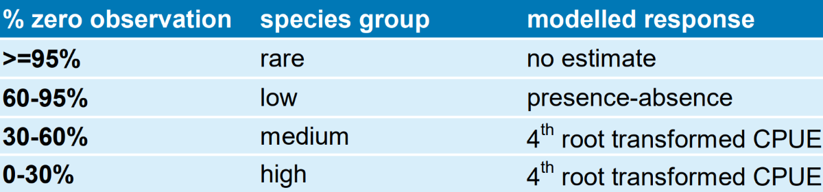
1. Determine rare, low, medium and high prevalent species
Whether a species is prevalent in the survey was determined by the percentage of zero observations (Table 8). Trends were not estimated for rare species (however, yearly averages plus standard deviation of raw data are presented); trends of presence-absence were estimated for low prevalence species, and trends of 4th root transformed CPUE were estimated for medium and high prevalence species.
Table 8. Definition of species prevalence
2. Model fitting and validation
A GAM was applied with year fitted as a thin plate regression spline. To account for depth-stratified sampling design, water depth was included as smoother in DFS and DYFS surveys. For presence-absence trend models, the response was modelled as a binomial distribution with a logit link function. For CPUE trend models, the response was modelled either as Gaussian distribution (with identity link) or Gamma distribution (with log link).
The number of basic functions (parameter k in the smoother) determines how much curvature the fitted year smoother shows. A k set too high could result in capturing unnecessary yearly fluctuations in CPUE. A k set too low could result in missing patterns. The choice of k depends on the total number of years in the survey and the scale of trends we expect to see. Several k values were tested, and we visually compared the detected trends to the raw data plots to select the k that gives the best shape/scale of the expected trend. In the end the k values were determined as: k=4 for surveys covering around 20 years; k=8 for surveys covering around 40 years.
Model diagnostics were conducted, including residual checking (plots and tests) and AIC. Models that did not fit well were marked (visible in light grey confidence intervals in the plots); the results of these models should be interpreted with more caution.
3. Determine significant trends based on the 1st derivative of the year smoother
The 1st derivative of the year was smoother, as well as the 98% simultaneous confidence interval, was calculated. Significantly increasing, decreasing or stable periods were then determined: a negative 1st derivative (including CI) defined a significantly decreasing period, while a positive 1st derivative (including CI) defined a significantly increasing period.
Due to the large sample size in the surveys, the significance level was increased from 0.95 to 0.98 compared to Trendspotter (with only small sample sizes). A statistically stable period was also determined: when the CI of the 1st derivative covered 0 and stayed within +/- 0.1. This period can be interpreted approximately as CPUE (transformed) changes of less than 10% per year. The trend class definitions used in this study are given in Table 9.
Table 9. Trend classification

Discussion
-
The GAM method results in more curved trends than the structure time-series analysis method. This is due to the flexibility in building curvature in splines.
-
GAM can only fit a smoothing changing process and therefore it is difficult to handle data with sudden large changes, such as several eel stocks in our study. In these cases, the catches of eel suddenly decreased to 0 since 2007.
-
In the few eel cases, since 2007, years are all zero observation. In this case, the estimated CI becomes very large. This is an artefact, rather than an actual large uncertainty.
-
The current model runs on the 4th root transformed raw data so that the trends represent the mean of the 4th root transformed CPUE, while in the previous study, trends represent the 4th root transformed annual mean CPUE.
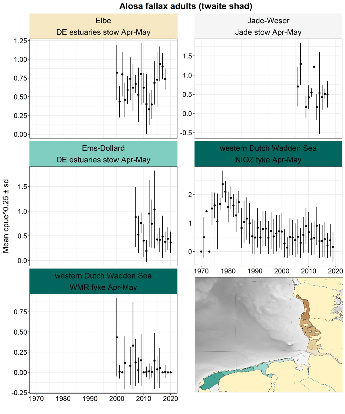
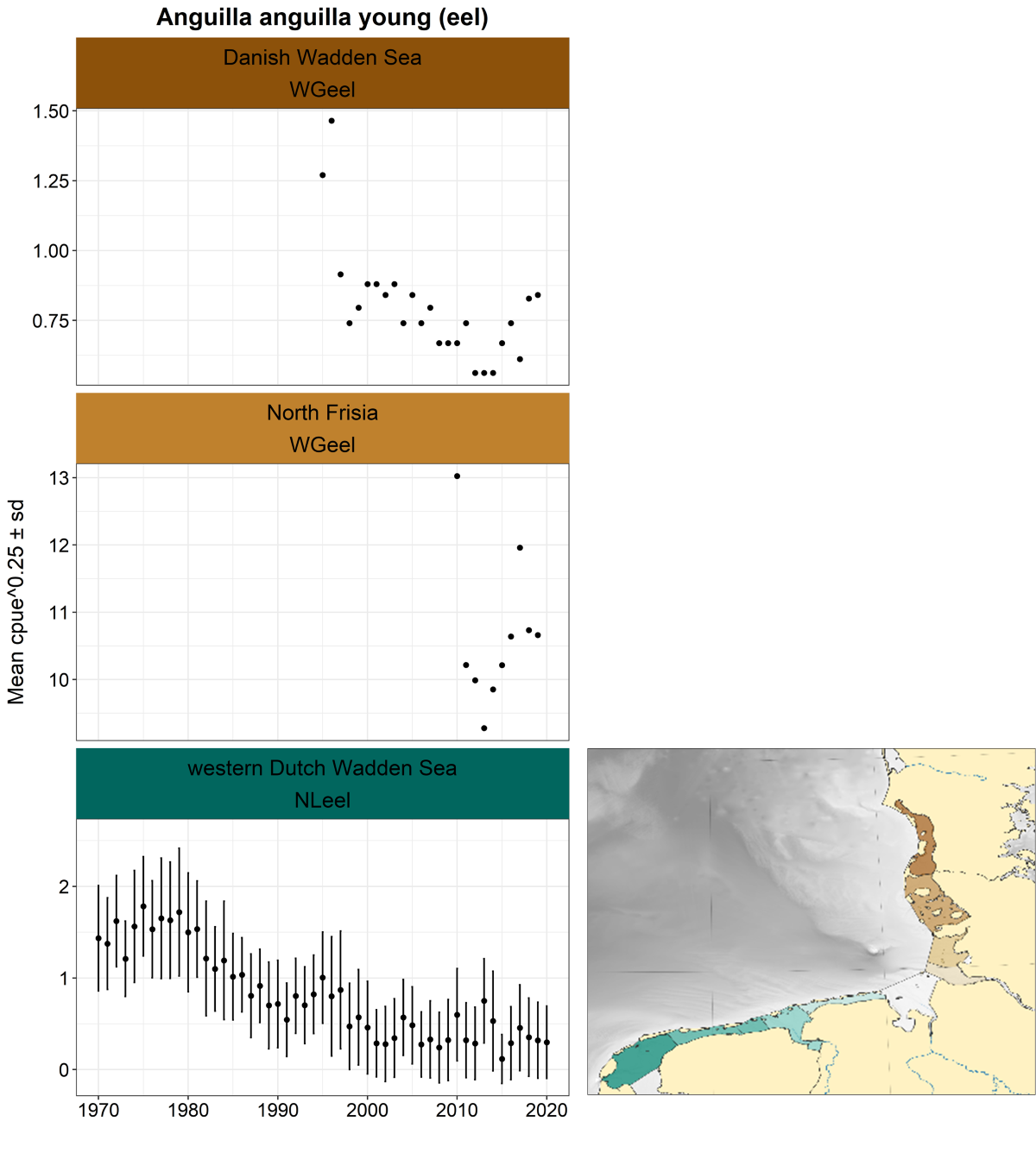
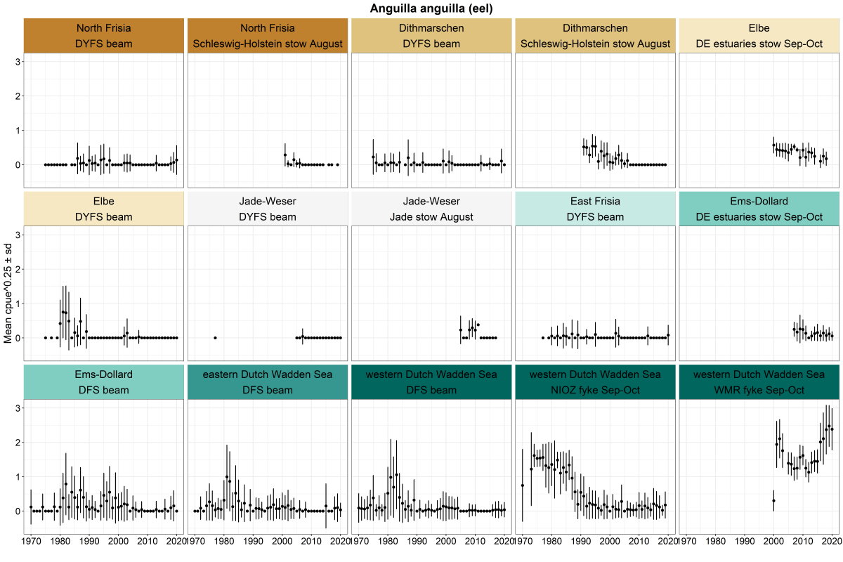
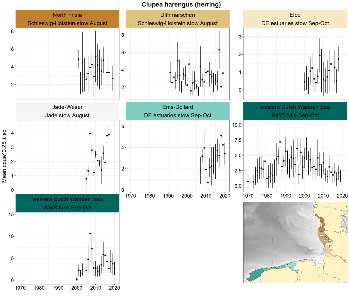
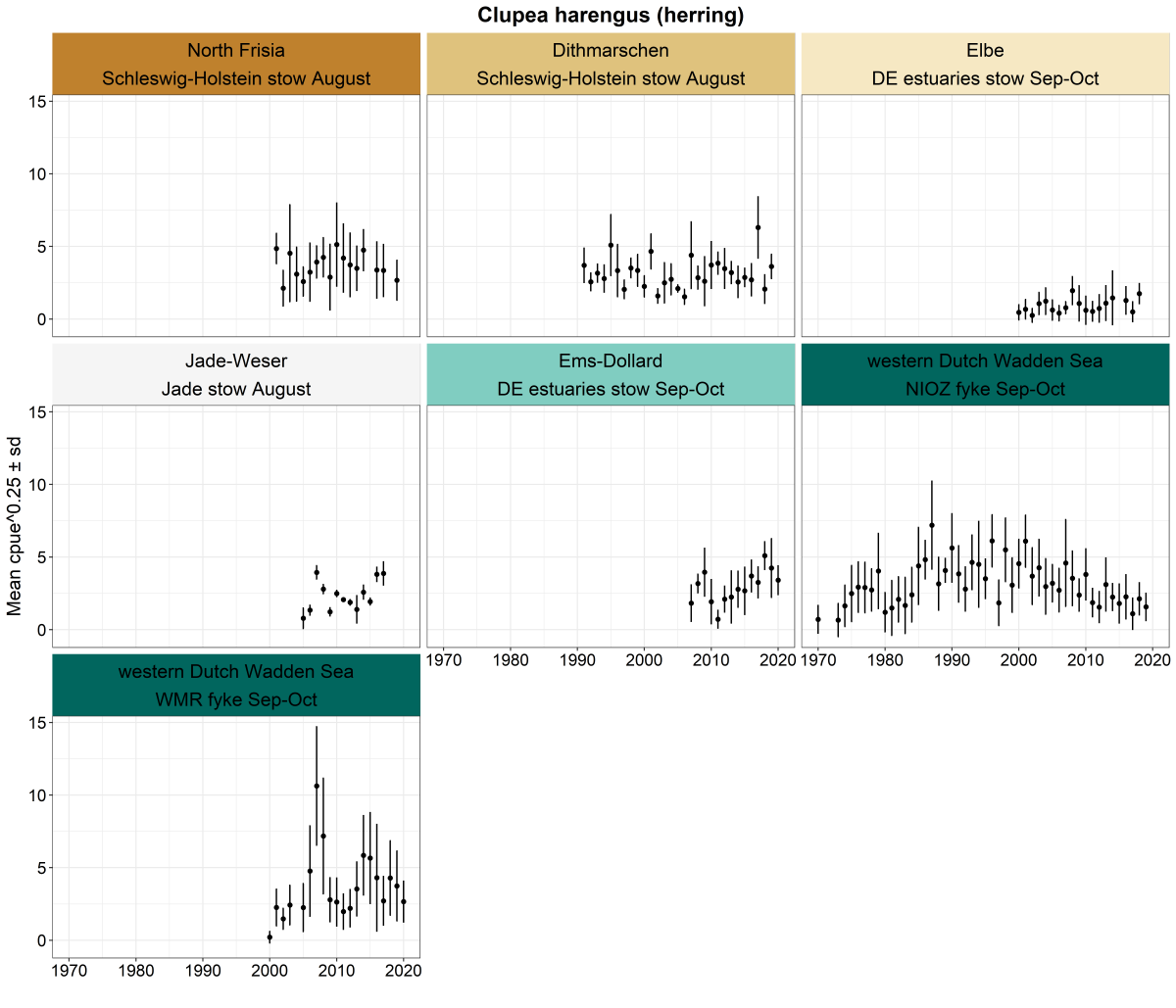
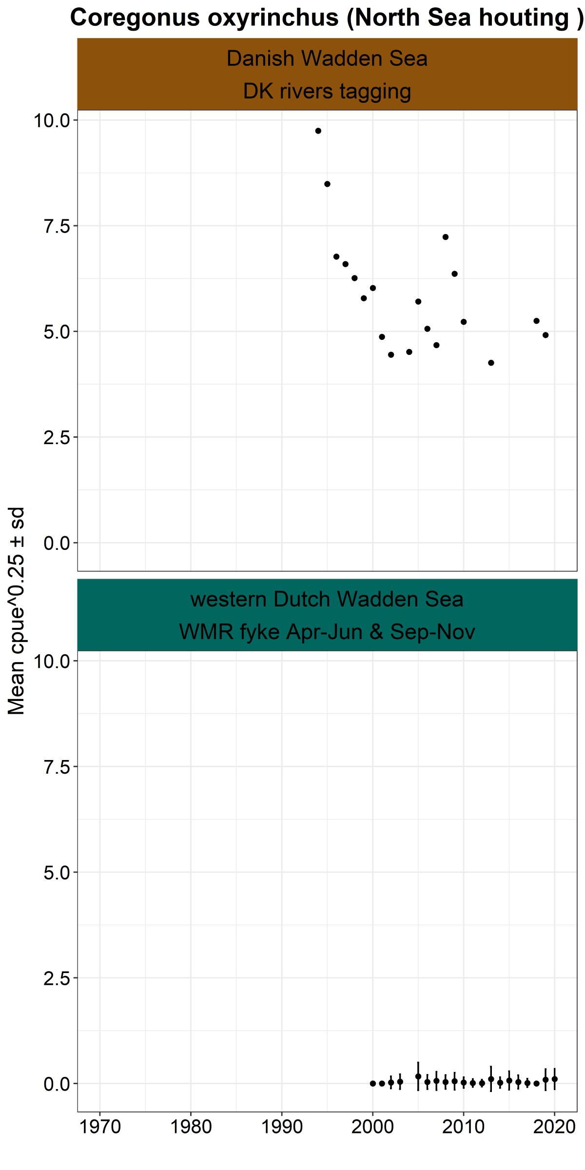
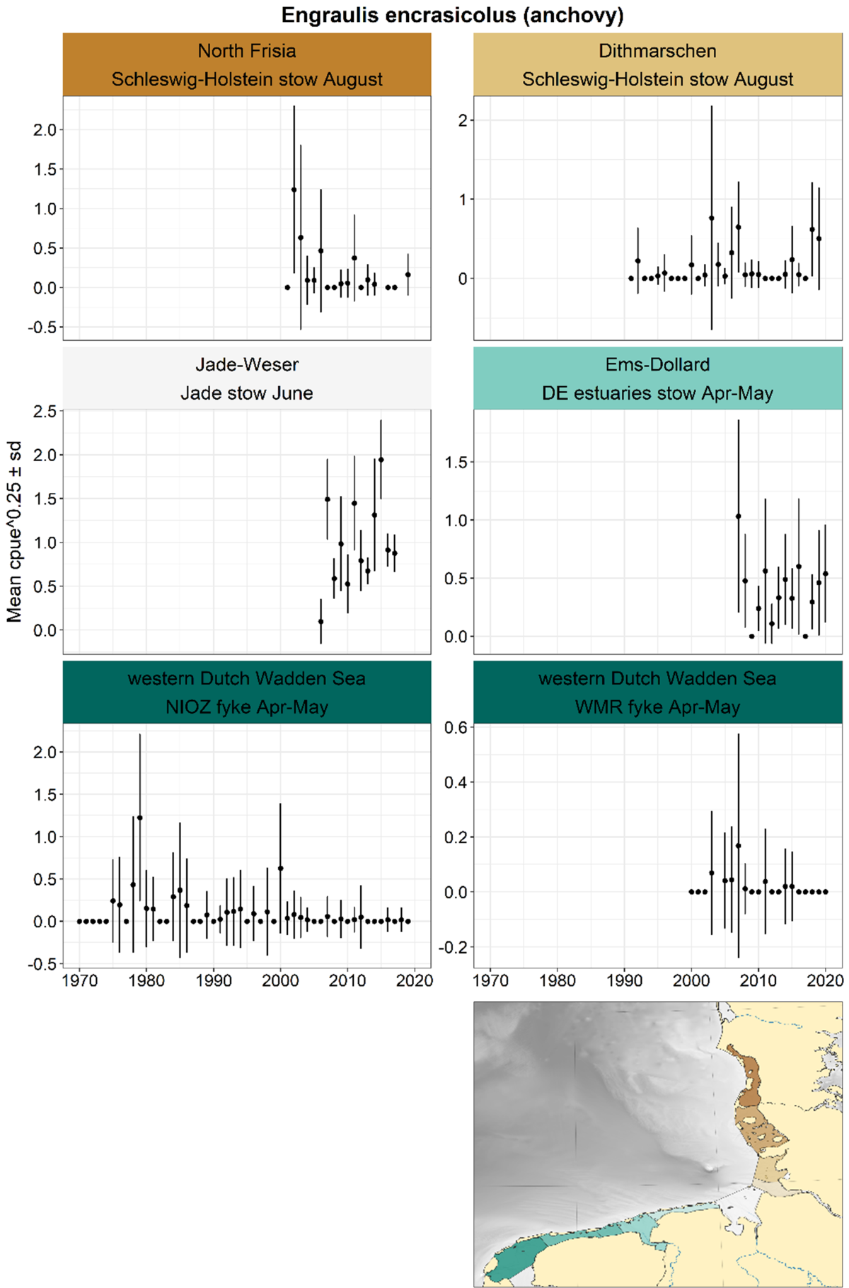
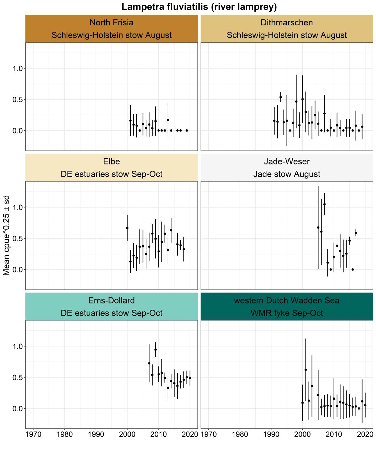
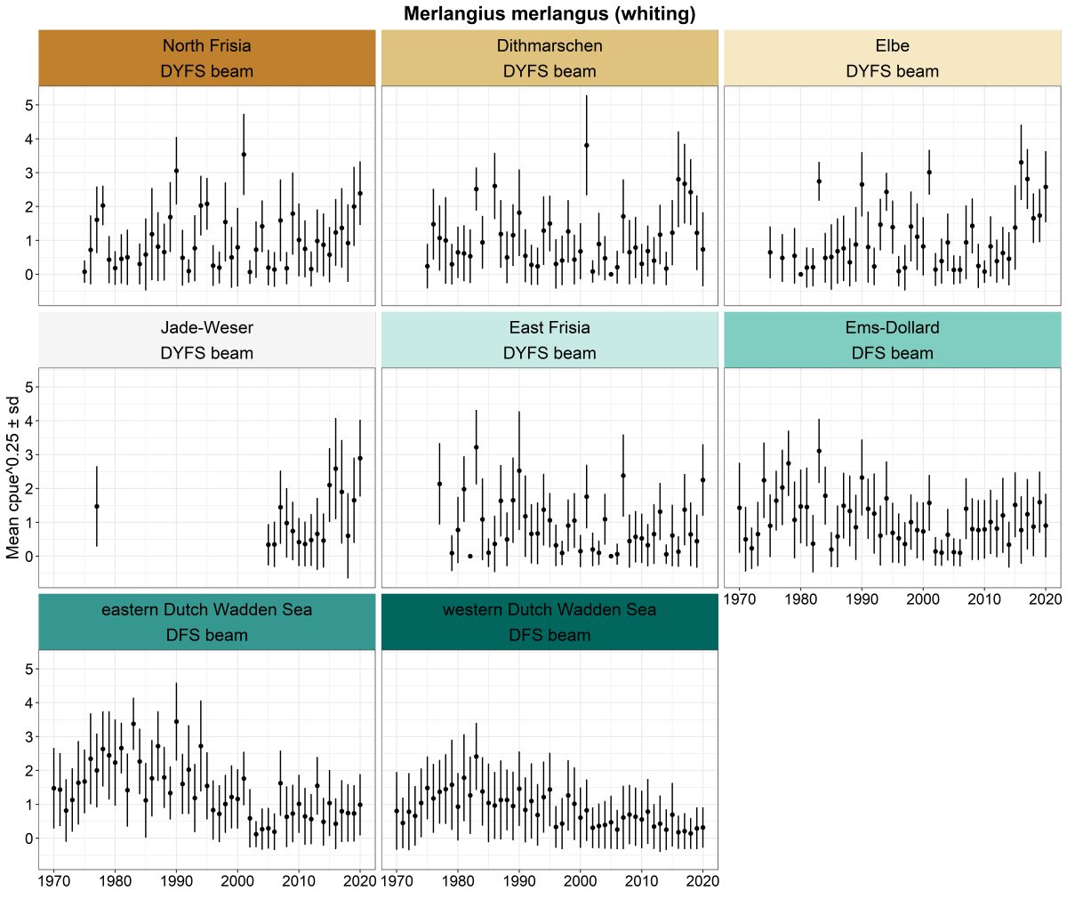
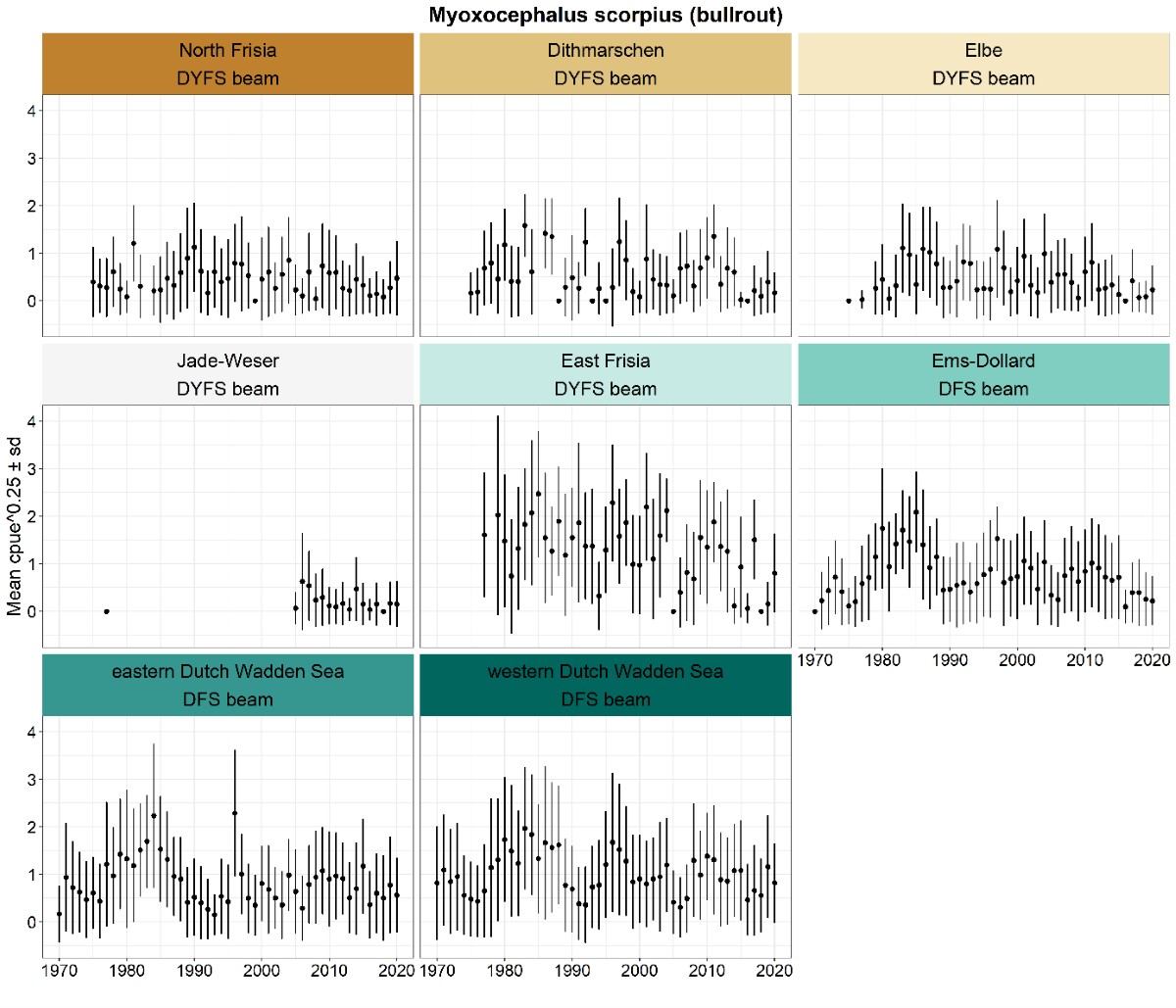
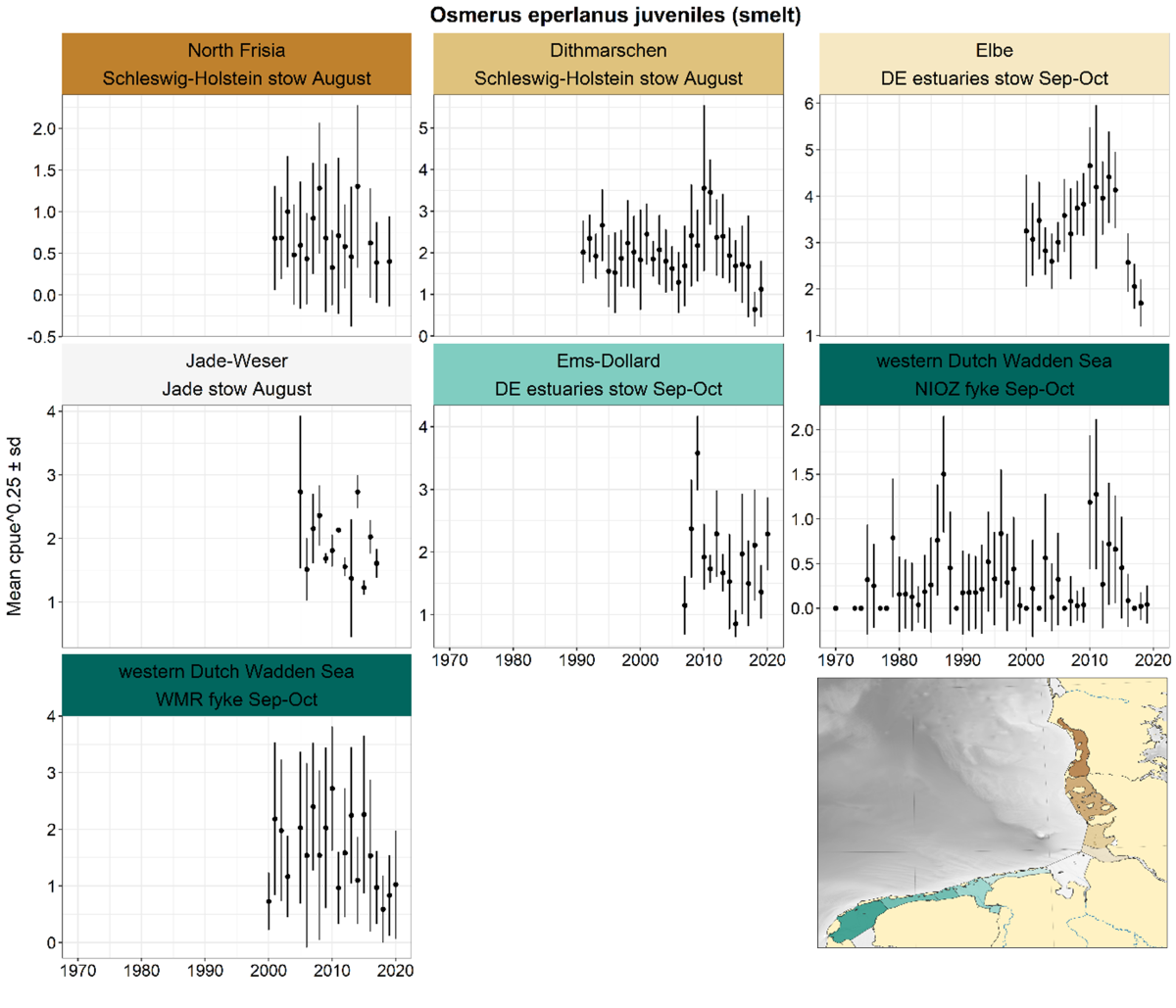
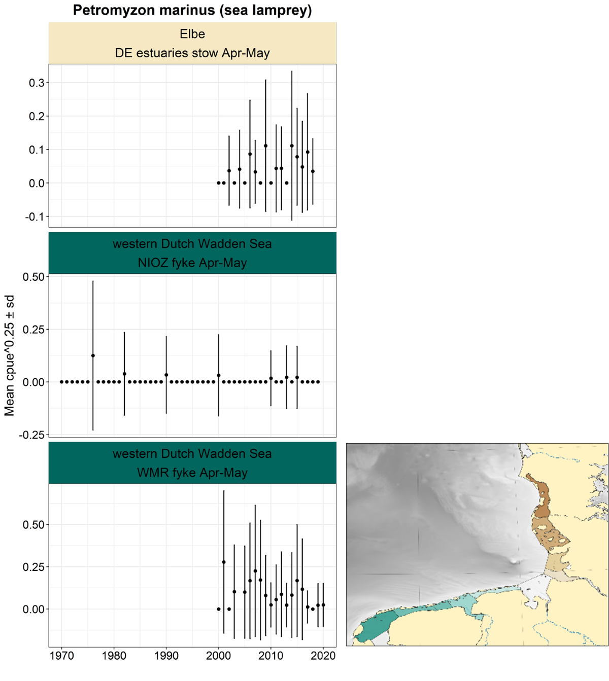
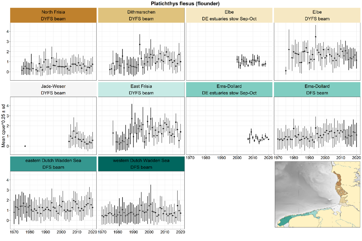
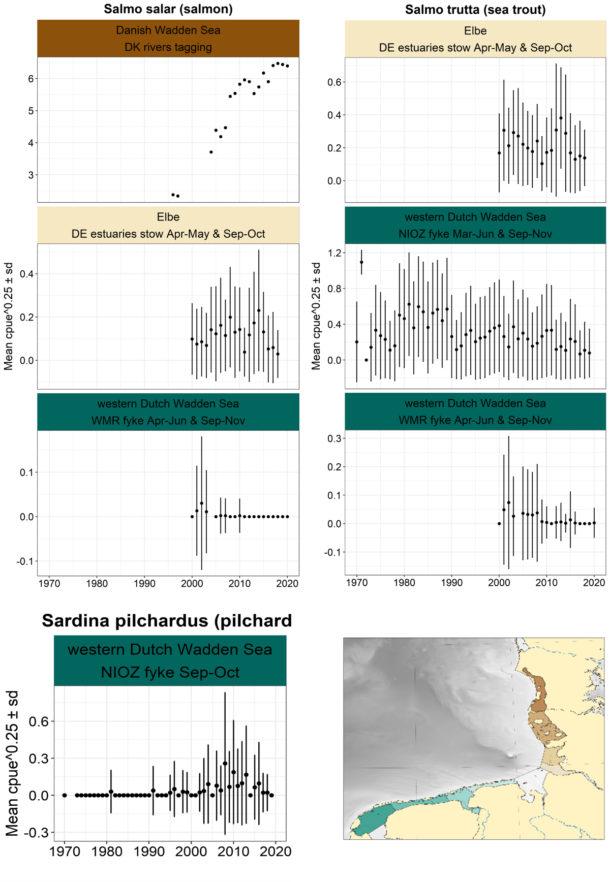
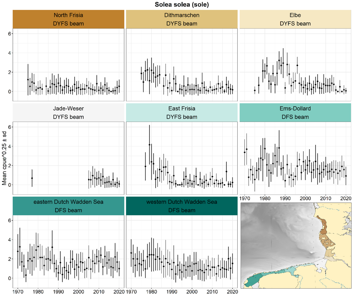
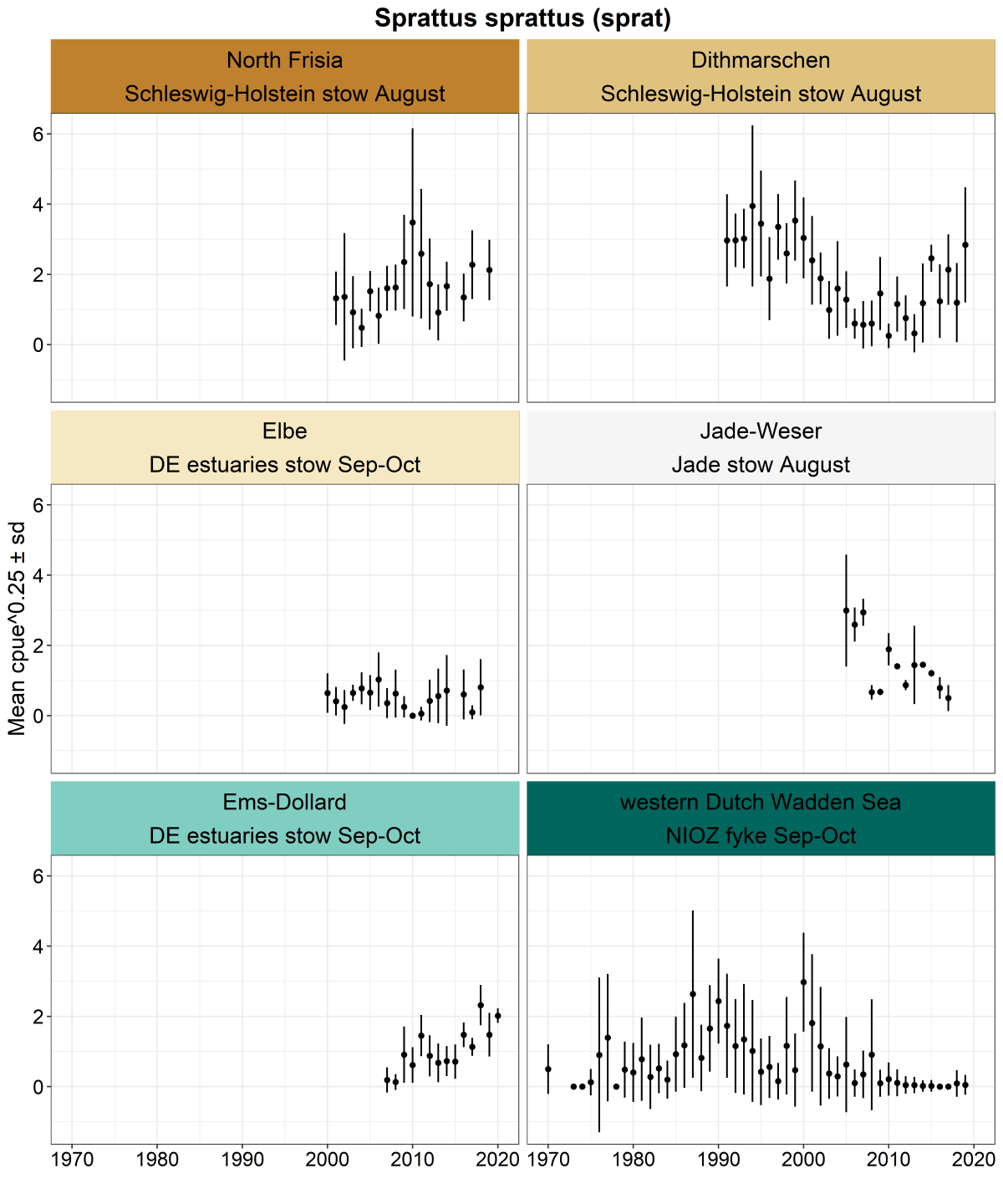
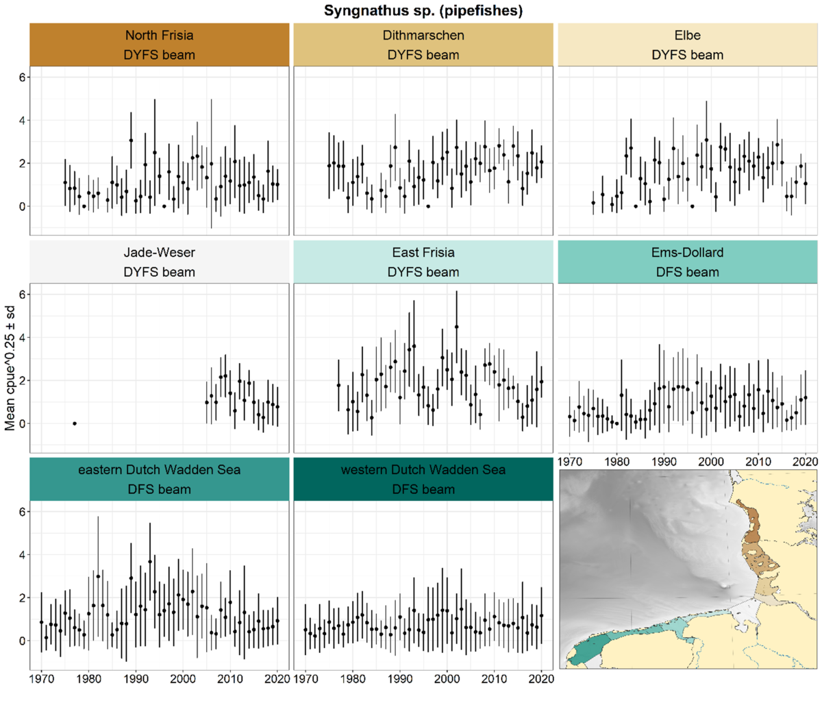
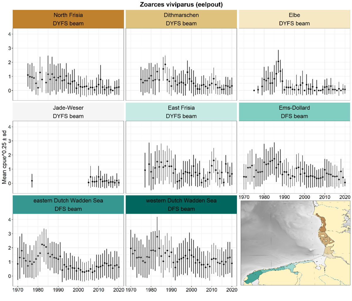
Annex 3: Plots of raw data
In alphabetical order, note the different y-axes for trends based on both stow net and fyke: since the measuring units differ (number per water volume and number per fyke days) values on y-axes cannot be compared.


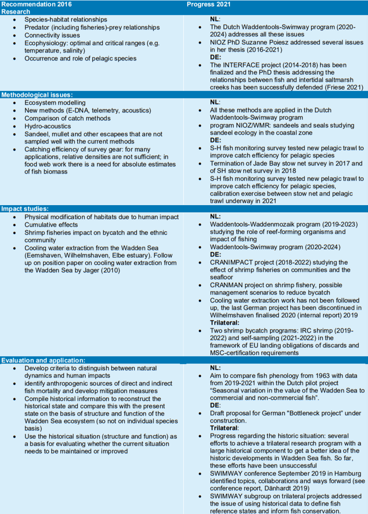
Annex 4: Evaluations of 2017 recommendations
Management

Monitoring & Research