1. Introduction

The Wadden Sea is an important area for many fish species. The shallow coastal area forms the transition between the estuaries and the North Sea (Figure 1). The inner Wadden Sea is connected with several estuaries, which are characterized by a pronounced salinity gradient. The outer Wadden Sea, demarked by the barrier islands, is connected with and influenced by the North Sea.
 
Many fish species rely on the Wadden Sea for at least one of their life stages. A suite of marine fish (flatfish, other groundfish and pelagic fish species) reach the Wadden Sea as post-larvae and spend their juvenile phase there (marine juveniles), benefitting from the high food availability and shelter from predators (van der Veer et al., 2000; Elliott et al., 2007). Other species inhabit the region en route to either marine or freshwater spawning sites (diadromous species), during certain times of the year (marine seasonal migrants) or only occasionally (marine adventitious species) (Elliott et al., 2007). Apart from the temporary visitors, the Wadden Sea is also inhabited by resident species that spend (almost) their entire life in the Wadden Sea.

Comprehensive lists of fish species occurring in the Wadden Sea have been published previously (Witte and Zijlstra, 1978; Bolle et al, 2009). In this report, we list all species observed in long-term monitoring programmes during the last decade. For the status and trends, we focus on a selection of species and functional groups, which are typically found in the Wadden Sea. We also discuss elasmobranchs and other rare species (paragraph 2). As the trilateral fish targets (CWSS, 2010) are described in an abstract manner, they cannot be evaluated quantitatively. Therefore, this report was restricted to describing and classifying trends. The trilateral targets are evaluated only in a qualitative way. However, we sketch how progress towards testable targets can be achieved (paragraph 3).

 

Figure 1. Tidal flat Ems estuary (Photo: Oscar Bos).

 

2. Status and trends

2.1 Selected monitoring programmes and species for trend analysis

The status and trends of the Wadden Sea fish are based on fish monitoring programmes covering a time span of at least ten years, up to the present (Table 1, Figure 2). Further details on the monitoring programmes are provided in Annex 1.

 

Table 1. Overview of the long-term fish monitoring programmes included in the trend analyses. The sampling areas are shown in Figure 2.

 

Figure 2. Map of the sampling areas and locations. The beam trawl surveys cover all sampling areas except the Danish Wadden Sea. The sampling locations of passive gears and the Danish rivers included in the tagging programme are indicated by symbols. The background colours of the sampling areas correspond with the strip colours in the trend figures.

 

Consistent with the previous Quality Status Report (QSR) (Tulp et al., 2017), species were selected to represent the three most important functional guilds in the Wadden Sea: marine juveniles, estuarine residents and diadromous species (Table 2). Sprat (Sprattus sprattus, marine adventitious) was included because it is an important prey item for birds. Anchovy (Engraulis encrasicolus) and pilchard (Sardina pilchardus, both belonging to the marine seasonal guild) were evaluated because these species are expected to increase in the Wadden Sea (Alheit et al., 2012; Tulp et al., 2017).

For most species, only the most suitable sampling method was chosen: beam trawl for demersal species, and stow net and fyke for pelagic species (Figure 3). For eel (Anguilla anguilla), both beam trawl and passive gears were used, and these data were further supplemented with estimates of juvenile eel from the NL glass eel survey and the ICES WGeel recruitment indices. For flounder (Platichthys flesus), the German estuaries stow net data were included because flounder is a typical species in transitional waters. Abundance estimates of diadromous species in Danish rivers were based on mark-recapture studies and sufficiently long time series were only available for salmon (Salmo salar) and the North Sea houting (Coregonus oxyrinchus). These two species, along with sea trout (Salmo trutta), were rare or absent in the stow net and fyke programmes.

All stow net and fyke programmes, except the Schleswig-Holstein stow net, were deployed for several months each year (Table 1). As seasonal patterns may confound annual patterns, we chose representative periods for most species (periods are indicated in the trend plots).

 

Table 2. Selected species by guild and sampling method. (X) = limited presence. 

 

 

Figure 3. Selected long-term monitoring programmes for Wadden Sea fish trend analysis include: Upper left (A) NIOZ fyke near Texel, The Netherlands (Photo: Lodewijk van Walraven); Upper right (B) Stownet fishing (Photo: Ralf Vorberg); Lower (C) Dutch Demersal Fish Survey (DFS) in the Wadden Sea (Photo: Ingrid Tulp). Further details on the monitoring programmes are provided in Annex 1.

 

2.2 Methods of trend analysis

For the standardised trend analysis, we used General Additive Models (GAMs). This approach differs from the method used in the 2017 QSR (Trendspotter, (Visser, 2004; Tulp et al., 2017)). GAMs share advantages with Trendspotter such as estimating flexible trends, trend classification and dealing with missing values. Instead of using annual means as input as required by Trendspotter, GAMs allow the use of the data at the observation level so that all individual samples can be used. This allows for reducing bias and variance in the year signal by accounting for covariates such as water depth or salinity. 

Two different response variables were used, depending on species occurrence (expressed as a percentage of zero observations). For common species, we modelled abundance estimates (catch per unit of effort (CPUE) for most surveys, absolute abundance estimates for Danish rivers and WGeel North Frisia). For less common species, the probability of occurrence was modelled. Abundance estimates were 4th-root transformed and modelled with either gamma or Gaussian distribution. Fourth-root transformation is commonly used for this type of data and has the advantage that it improves the interpretation of trend figures and that zero values can be dealt with more easily than when using a log transformation. The probability of occurrence was modelled with a binomial distribution. The response variable (abundance or probability of occurrence) is given in the top right corner of each plot.

The following cut-off values between the two approaches were applied:

•  <30 % zero observations => high abundance  => abundance modelling
• 30-60 % zero observations  => intermediate abundance => abundance modelling
• 60-95 % zero observations  => low abundance => probability of occurrence modelling
• >95 % zero observations => rare species  => no estimate

For the beam trawl surveys (DFS and DYFS) water depth was included as a covariate. The resulting trend plots show the estimated trends at median depth. For the German estuaries stow net sampling, salinity was included as a categorical covariate with 3 levels (oligo-, meso- and polyhaline). For the latter areas, trend plots depict the trend at intermediate (mesohaline) salinity. The y-values in the plots can therefore not be interpreted as absolute values (and are not directly comparable between areas) but can only be used to describe trends.

Trends were classified per year and visualised in the plots according to the following classification:

 

Colour Legend for trend classification in Figures 4 - 32

 

Model fit was assessed through residual plots, model AIC and comparison with raw data. For abundance modelling, the decision for gamma or Gaussian distribution was also based on this assessment. In case the model fit was insufficient based on the above criteria, the confidence interval was coloured light grey in the trend figures. For further methodological details of trend calculation and classification see Annex 2.

Model outcomes were summarised by decade and larger regions by taking the statistical model of the trend scores (increase, decrease, stable or uncertain) by year and area. For the summary, the areas were aggregated to the Dutch Wadden Sea, the German Wadden Sea and the Danish rivers.

Because we realise there is an interest in examining the actual values, plots of the raw data (yearly means ± standard deviation) are also presented (Annex 3). Abundance estimates of raw data were 4th root transformed before averaging.

As a result of the new approach used for the analyses, the following differences with the trend graphs from the previous QSR report (Tulp et al., 2017) must be considered:

• The GAM method results in more curved trends than the Trendspotter trends. This is due to the flexibility in building curvature in splines.

• The current model runs on the 4th root transformed raw data, so the trends represent the mean of the 4th root transformed data, while in the previous report, trends represented the 4th root transformed annual mean. 

• We now use two types of response variables: abundance estimates for the common species/area combinations and probability of occurrence for the rarer species. In the previous QSR, we only used abundance estimates.

• Compared to the previous report, in several species, more periods are classified as stable instead of uncertain. This is due to the fact that we now use the individual samples and covariates, so we can account for variation much better.

The methodological development added considerable robustness, detail and transparency to the analyses, while at the same time hampering comparability with earlier analyses. Therefore, we did not include a comparison of trends between the QSR thematic reports 2005, 2009, 2017 and 2022.

 

2.3 Trend analysis for selected species

Species were grouped to illustrate trends by the functional guilds (Elliott & Hemingway, 2002, Table 2). For marine juveniles and estuarine resident species, the overall trend of the functional guild was analysed based on DFS and DYFS data. For the other functional guilds, data and number of species were too limited for a guild specific analysis. 

2.3.1 Marine juvenile species

Marine juveniles showed declines in nearly all subareas since the early or mid-1980s, followed by a subsequent stabilisation at a low level in the one to two most recent decades (Figure 4). The exception to this pattern is the Elbe. The seemingly upward trend during the last five years in North Frisia, East Frisia and Jade-Weser was classified as uncertain (black) or stable (yellow) because of large year-to-year variation.

 

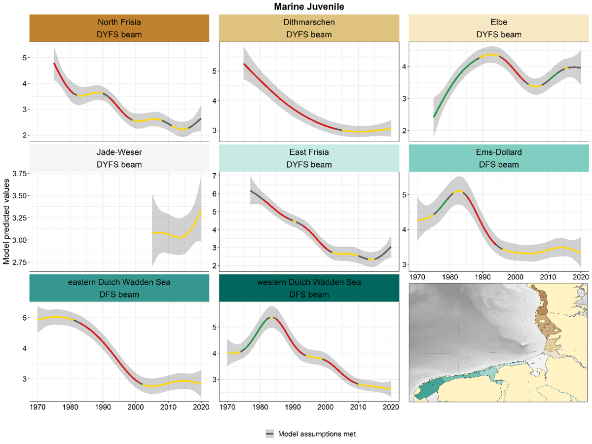Figure 4. Trends in modelled predicted abundance of marine juvenile species in the different areas. Trend lines represent GAM models. The model predicted values (in this case densities) are on the y-axes. The grey shaded area represents the confidence interval; if the shaded area is dark grey the model assumptions are met, in the case of a light grey shaded area the model assumptions are not met. Colour coding for the trend line: red-decrease, green-increase, yellow-stable, grey-uncertain. Because model predictions are given for a mean depth per area absolute y-values are not comparable between areas.

 

2.3.1.1 Pleuronectes platessa - plaice

Plaice declined in most areas and surveys since the 1980s, with stable periods and periods of decline alternating and varying between areas (Figure 5). The Elbe is an exception to this pattern: an increase until 1990 and a stabilisation thereafter. Although not significant, trends made an upward bend in the German areas in the past five years.

 

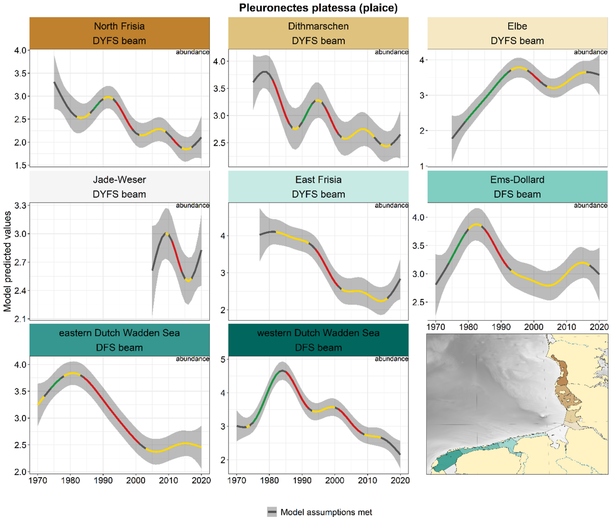Figure 5. Trends in modelled predicted abundance/probability of occurrence of plaice in the different areas. The area-specific response variable is indicated in the top right corner of each panel. Trend lines represent GAM models. The model predicted values are on the y-axes. The grey shaded area represents the confidence interval; if the shaded area is dark grey the model assumptions are met, in the case of a light grey shaded area the model assumptions are not met. Colourcoding for the trend line: red-decrease, green-increase, yellow-stable, grey-uncertain. Because model predictions are given for a mean depth per area absolute y-values are not comparable between areas.

 

2.3.1.2 Solea solea - sole

Sole showed peaks between 1975 and 1985 in most areas, followed by a decrease (Figure 6). While levels have stayed low in the German areas, numbers have increased in the Dutch areas after the absolute low in the 1990s. In the Dutch areas shorter periods of in- and decreases occurred since the 1990s.

 

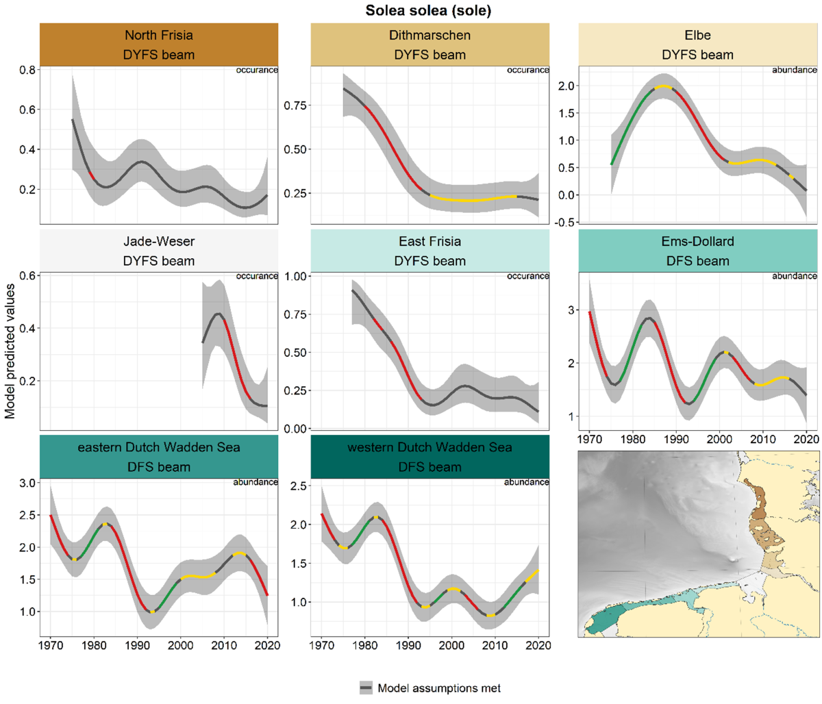Figure 6. Trends in modelled predicted abundance/probability of occurrence of sole in the different areas. The area-specific response variable is indicated in the top right corner of each panel. Trend lines represent GAM models. The model predicted values are on the y-axes. The grey shaded area represents the confidence interval; if the shaded area is dark grey the model assumptions are met, in the case of a light grey shaded area the model assumptions are not met. Colourcoding for the trend line: red-decrease, green-increase, yellow-stable, grey-uncertain. Because model predictions are given for a mean depth per area absolute y-values are not comparable between areas.

 

2.3.1.3 Limanda limanda - dab

Of all marine juvenile species, dab showed the strongest declines. Since the 1980s, dab declined in most areas and surveys (Figure 7). The one exception to this pattern is the Jade-Weser, with alternating periods of significant de- and increase. In the eastern and western Dutch Wadden Sea there was a recent upward bend in the trend, although not significant.

 

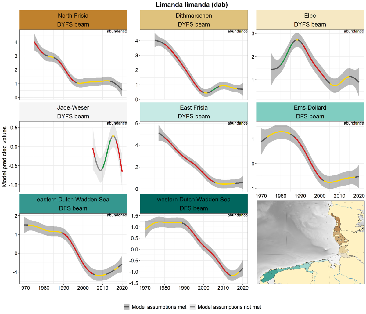Figure 7. Trends in modelled predicted abundance/probability of occurrence of dab in the different areas. The area-specific response variable is indicated in the top right corner of each panel. Trend lines represent GAM models. The model predicted values are on the y-axes. The grey shaded area represents the confidence interval; if the shaded area is dark grey the model assumptions are met, in the case of a light grey shaded area the model assumptions are not met. Colourcoding for the trend line: red-decrease, green-increase, yellow-stable, grey-uncertain. Because model predictions are given for a mean depth per area absolute y-values are not comparable between areas.

 

2.3.1.4 Merlangius merlangus - whiting

Whiting showed different trends in different subareas with a clear distinction between the German and Dutch areas (Figure 8). After an initial increase until 1980, densities collapsed in all Dutch areas until the early 2000s, after which they stabilised. In the German areas, trends were more stable during the period 1975-2010, with exception of Dithmarschen with strong up-and-down trends. Since ca. 2010, there was a clear increase in all German areas.

 

Figure 8. Trends in modelled predicted abundance/probability of occurrence of whiting in the different areas. The area-specific response variable is indicated in the top right corner of each panel. Trend lines represent GAM models. The model predicted values are on the y-axes. The grey shaded area represents the confidence interval; if the shaded area is dark grey the model assumptions are met, in the case of a light grey shaded area the model assumptions are not met. Colourcoding for the trend line: red-decrease, green-increase, yellow-stable, grey-uncertain. Because model predictions are given for a mean depth per area absolute y-values are not comparable between areas.

 

2.3.1.5 Gadus morhua - cod

Cod showed a negative trend in all areas and surveys from 1980 onwards, within some areas intermediate periods with increasing trends (e.g. 1990-2000 North Frisia, Elbe) (Figure 9).

 

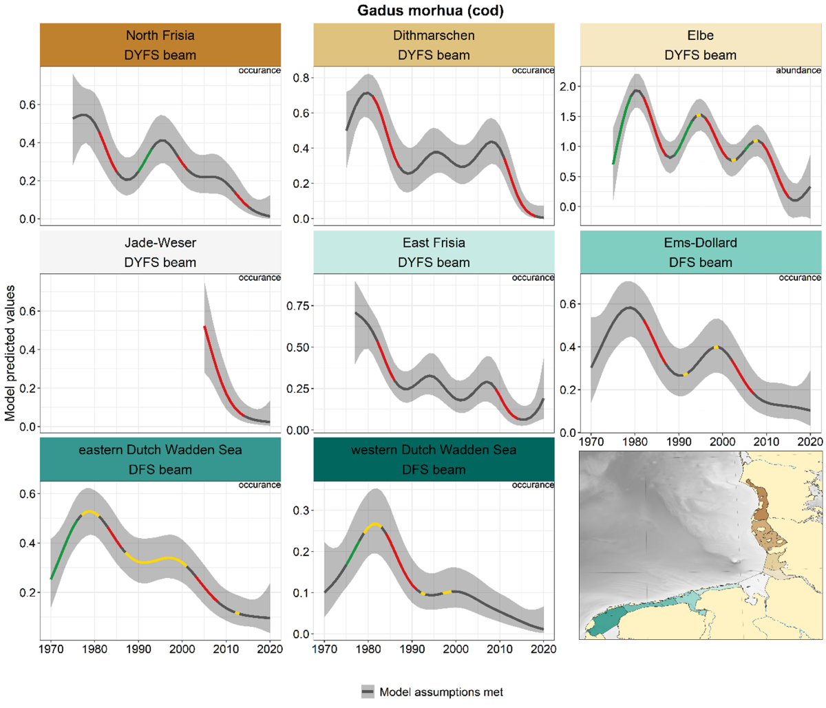Figure 9. Trends in modelled predicted abundance/probability of occurrence of cod in the different areas. The area-specific response variable is indicated in the top right corner of each panel. Trend lines represent GAM models. The model predicted values are on the y-axes. The grey shaded area represents the confidence interval; if the shaded area is dark grey the model assumptions are met, in the case of a light grey shaded area the model assumptions are not met. Colour coding for the trend line: red-decrease, green-increase, yellow-stable, grey-uncertain. Because model predictions are given for a mean depth per area absolute y-values are not comparable between areas.

 

2.3.1.6 Chelidonichthys lucerna - tub gurnard

Trends in tub gurnard were highly uncertain in all areas for most of the time period, partly because of low catch rates (hence only estimation of presence/absence, Figure 10). Around 1980, tub gurnard only occurred in the most south-westerly areas (Dutch Wadden Sea). In several areas, there was a steep increase after 2000-2005 until 2005-2015, after which densities decreased again (although only significant in the eastern Dutch Wadden Sea). 

 

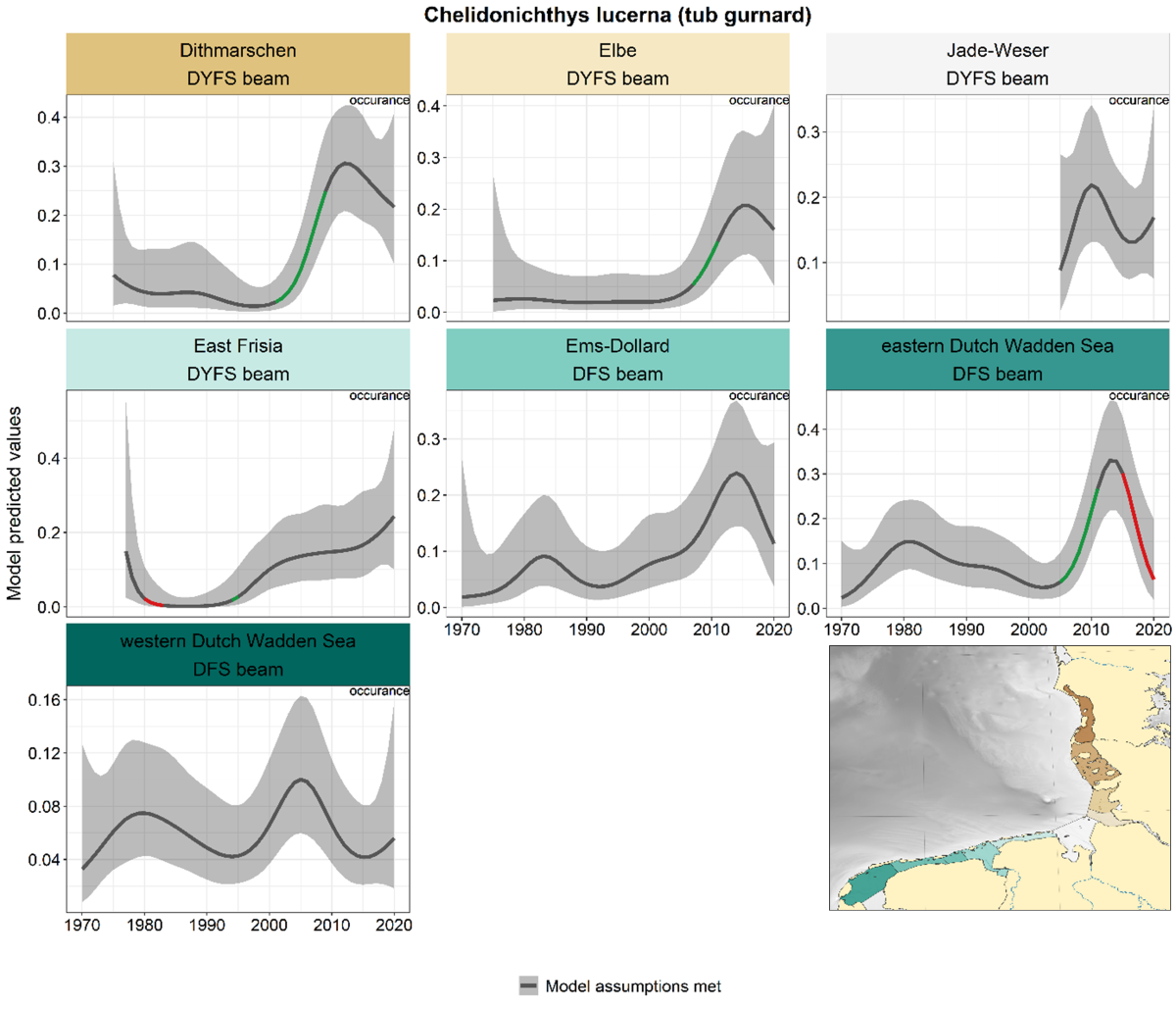Figure 10. Trends in modelled predicted abundance/probability of occurrence of tub gurnard in the different areas. The area-specific response variable is indicated in the top right corner of each panel. Trend lines represent GAM models. The model predicted values are on the y-axes. The grey shaded area represents the confidence interval; if the shaded area is dark grey the model assumptions are met, in the case of a light grey shaded area the model assumptions are not met. Colour coding for the trend line: red-decrease, green-increase, yellow-stable, grey-uncertain. Because model predictions are given for a mean depth per area absolute y-values are not comparable between areas.

 

2.3.1.7 Dicentrarchus labrax - sea bass

Trend information on sea bass is limited to three-time series (Figure 11). In the NIOZ fyke, sea bass showed an increasing trend from the 1980s until 2000, after a slight decrease, stabilising in the last decade. In the WMR fyke numbers are decreasing from 2005 onwards, while the occurrence in the Ems-Dollard is uncertain, but indicates a slight (nonsignificant) increase over the last decade. 

 

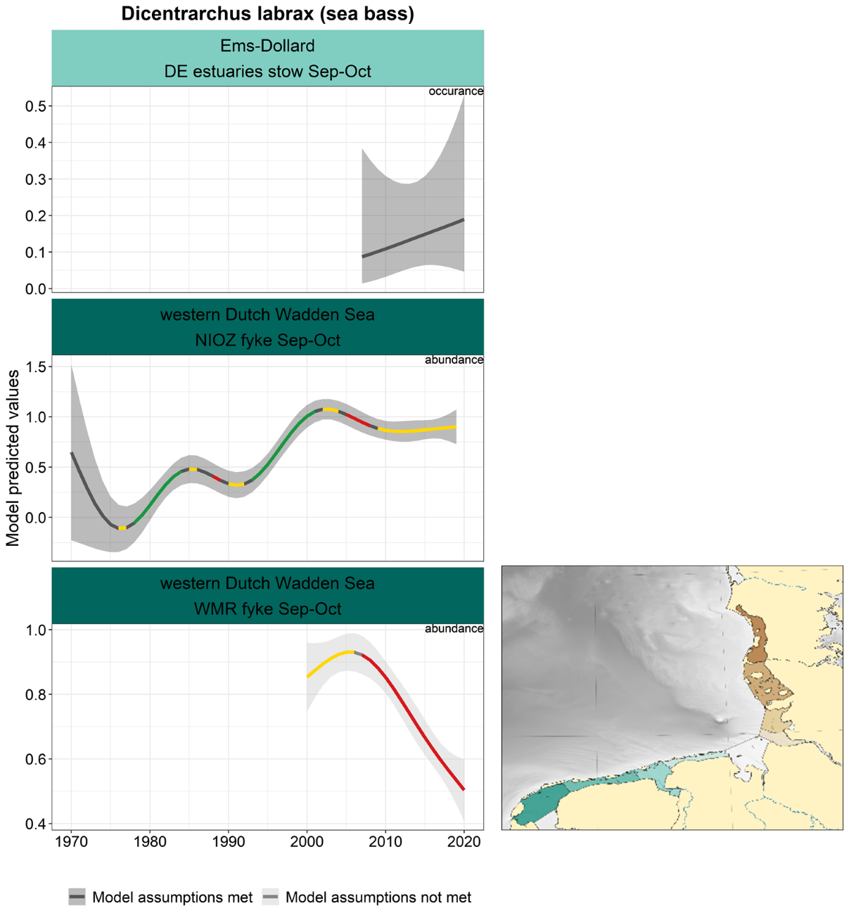Figure 11. Trends in modelled predicted abundance/probability of occurrence of sea bass in the different areas. The area-specific response variable is indicated in the top right corner of each panel. Trend lines represent GAM models. The model predicted values are on the y-axes. The grey shaded area represents the confidence interval; if the shaded area is dark grey the model assumptions are met, in the case of a light grey shaded area the model assumptions are not met. Colour coding for the trend line: red-decrease, green-increase, yellow-stable, grey-uncertain. Because model predictions are given for a mean depth per area absolute y-values are not comparable between areas.

 

2.3.1.8 Clupea harengus - herring

Information on herring was derived from fyke- and stow net monitoring. Along with sprat, anchovy and sardine, herring belongs to the so-called small pelagic fish species that generally live in schools. Trends for herring vary between the different areas (Figure 12). In the NIOZ fyke, herring showed a significant increase from the 1980s until 1990, followed by stabilisation, and a decline after 2005. In the WMR fyke, abundance increased from 2000 to 2010 followed by a decrease. In the Jade-Weser and Ems-Dollard, the trend increased over the last decade. In North Frisia, Dithmarschen and Elbe the trends were classified as stable or uncertain. 

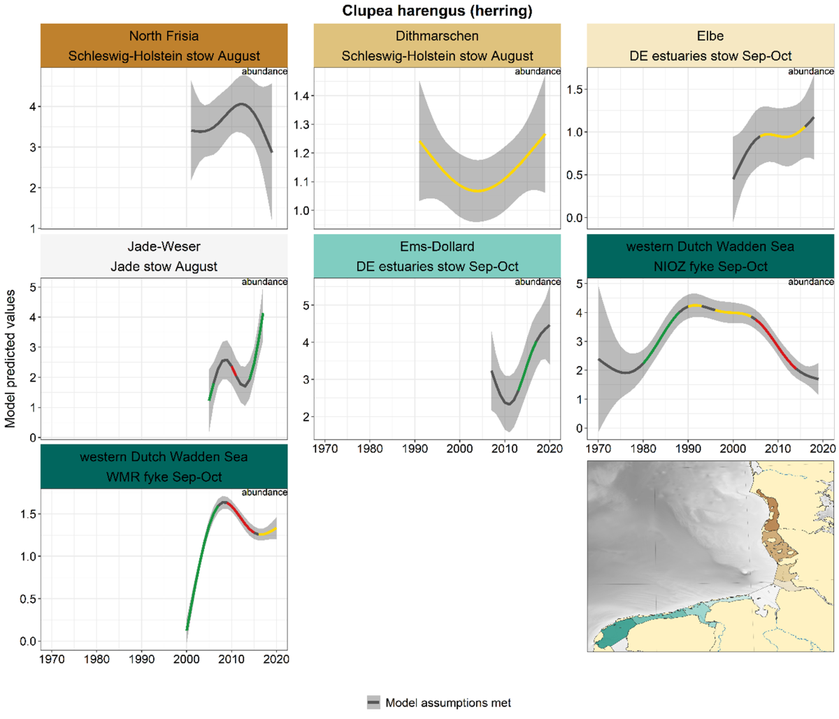Figure 12. Trends in modelled predicted abundance/probability of occurrence of herring in the different areas. The area-specific response variable is indicated in the top right corner of each panel. Trend lines represent GAM models. The model predicted values are on the y-axes. The grey shaded area represents the confidence interval; if the shaded area is dark grey the model assumptions are met, in the case of a light grey shaded area the model assumptions are not met. Colourcoding for the trend line: red-decrease, green-increase, yellow-stable, grey-uncertain. Because model predictions are given for a mean depth per area absolute y-values are not comparable between areas.

 

2.3.2 Estuarine resident species

Trends in estuarine species were highly variable across areas and surveys (Figure 13). Significant in- or decreases occurred in various periods in nearly all areas, but hardly ever at the same time. Since 2010 strong negative trends occurred in several German areas (Dithmarschen, Elbe and Jade-Weser), while in other areas the trends were more stable in the same period. The pattern in the western Dutch Wadden Sea was quite different from the other areas, with several alternating periods of in- and decreases. 

 

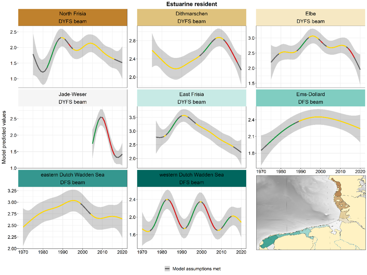Figure 13. Trends in modelled predicted abundance of estuarine residents in the different areas. Trend lines represent GAM models. The model predicted values (in this case densities) are on the y-axes. The grey shaded area represents the confidence interval; if the shaded area is dark grey the model assumptions are met, in the case of a light grey shaded area the model assumptions are not met. Colour coding for the trend line: red-decrease, green-increase, yellow-stable, grey-uncertain. Because model predictions are given for a mean depth per area absolute y-values are not comparable between areas.

 

2.3.2.1 Platichthys flesus - flounder

Flounder does not show a clear overall trend and few similarities across areas (Figure 14). Trends in many areas were characterised by long periods of stable or uncertain trends. A period with a significant increase occurred during 1990-2000 in North Frisia, Dithmarschen, Ems-Dollard and the western Dutch Wadden Sea.

 

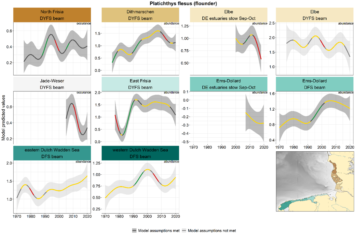Figure 14. Trends in modelled predicted abundance/probability of occurrence of flounder in the different areas. The area-specific response variable is indicated in the top right corner of each panel. Trend lines represent GAM models. The model predicted values are on the y-axes. The grey shaded area represents the confidence interval; if the shaded area is dark grey the model assumptions are met, in the case of a light grey shaded area the model assumptions are not met. Colour coding for the trend line: red-decrease, green-increase, yellow-stable, grey-uncertain. Because model predictions are given for a mean depth per area absolute y-values are not comparable between areas.

 

2.3.2.2 Zoarces viviparus - eelpout 

The overall trends showed similar patterns across areas (Figure 15). An initial increase until ca. 1985 was followed by a decline until ca. 2000. In most German areas the trend was either uncertain or stable after that, but in the Dutch areas, abundance started fluctuating with alternating periods of in- and decreases in similar periods.

 

Figure 15. Trends in modelled predicted abundance/probability of occurrence of eelpout in the different areas. The area-specific response variable is indicated in the top right corner of each panel. Trend lines represent GAM models. The model predicted values are on the y-axes. The grey shaded area represents the confidence interval; if the shaded area is dark grey the model assumptions are met, in the case of a light grey shaded area the model assumptions are not met. Colour coding for the trend line: red-decrease, green-increase, yellow-stable, grey-uncertain. Because model predictions are given for a mean depth per area absolute y-values are not comparable between areas.

 

2.3.2.3 Myoxocephalus scorpius - bull-rout

The same increase as observed in many other species until ca. 1980 was also observed in bull-rout (Figure 16). The occurrence of highs and lows strongly resembled those of eelpout. In general, the species is more abundant in the western area, hence abundance trends in the Dutch areas and presence/absence trends in the German area. The general pattern in the German areas was a decline from the 1980s onwards (although not classified as a significant decrease in all areas). The three Dutch DFS areas showed similar fluctuations with peaks around 1985, 2000 and 2015. 

 

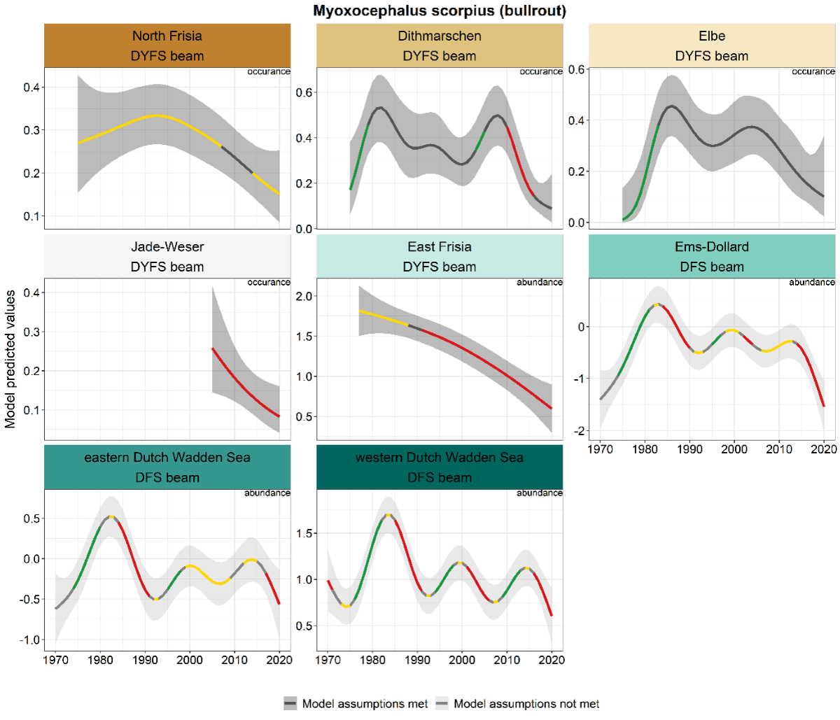Figure 16. Trends in modelled predicted abundance/probability of occurrence of bull-rout in the different areas. The area-specific response variable is indicated in the top right corner of each panel. Trend lines represent GAM models. The model predicted values are on the y-axes. The grey shaded area represents the confidence interval; if the shaded area is dark grey the model assumptions are met, in the case of a light grey shaded area the model assumptions are not met. Colourcoding for the trend line: red-decrease, green-increase, yellow-stable, grey-uncertain. Because model predictions are given for a mean depth per area absolute y-values are not comparable between areas.

 

2.3.2.4 Ciliata mustela - five bearded rockling

In several areas, an increase was observed between ca. 1990 and 2000. This increase was followed by a further increase in the western Dutch Wadden Sea, a decline in East Frisia, a stable trend in the eastern Dutch Wadden Sea and Ems-Dollard and an uncertain trend in the Elbe (Figure 17). In the two most northern Wadden Sea areas the trends are characterised by long periods of stable or uncertain trends. The trends in Jade-Weser and Elbe corresponded, with a decrease after 2010 and an increase in the past five years, but only the decrease in Jade-Weser was significant.

 

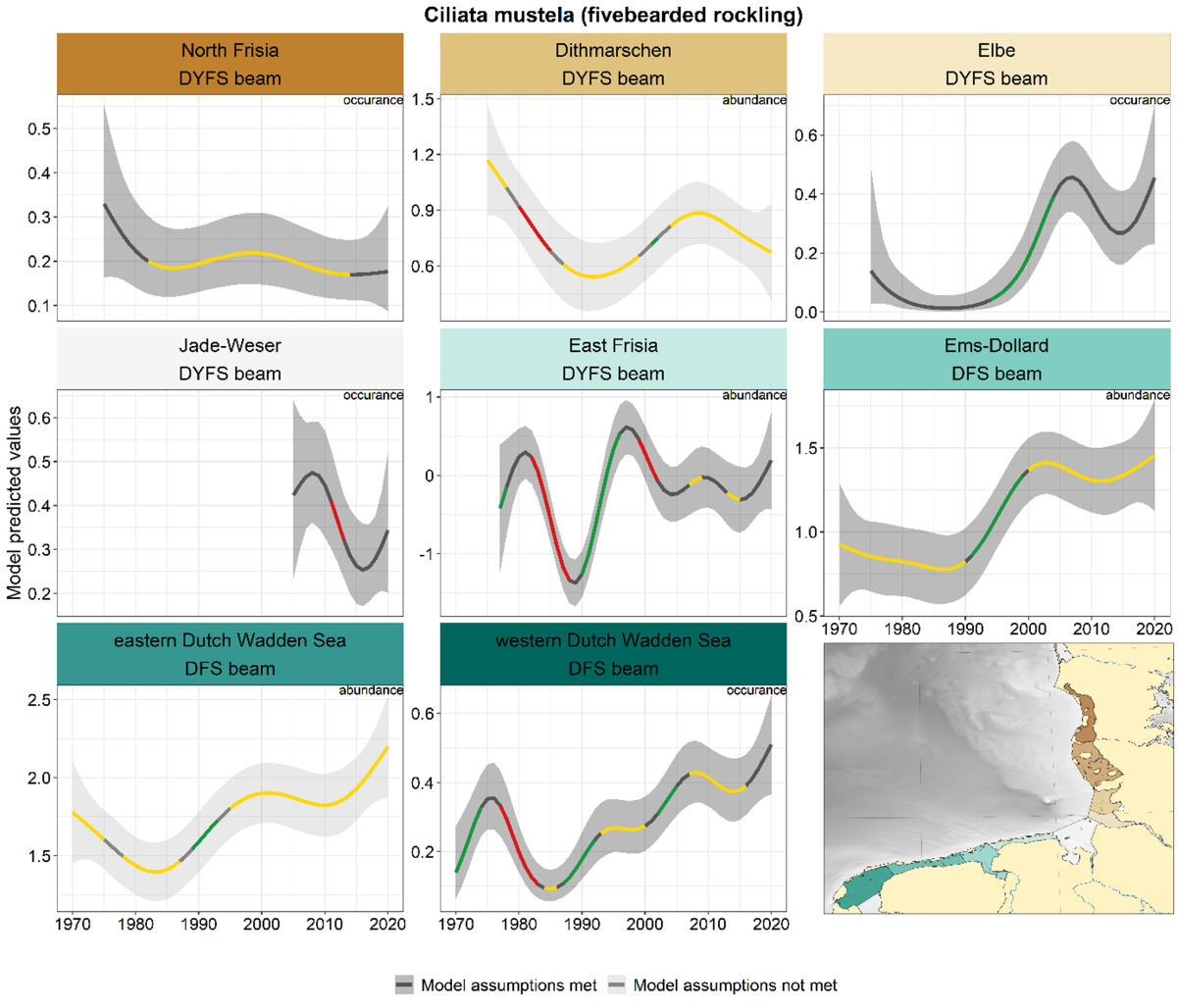Figure 17. Trends in modelled predicted abundance/probability of occurrence of fivebearded rockling in the different areas. The area-specific response variable is indicated in the top right corner of each panel. Trend lines represent GAM models. The model predicted values are on the y-axes. The grey shaded area represents the confidence interval; if the shaded area is dark grey the model assumptions are met, in the case of a light grey shaded area the model assumptions are not met. Colourcoding for the trend line: red-decrease, green-increase, yellow-stable, grey-uncertain. Because model predictions are given for a mean depth per area absolute y-values are not comparable between areas.

 

2.3.2.5 Agonus cataphractus - hooknose

The trends of hooknose are characterised by alternating periods of in- and decreases in all areas, that only occasionally coincided across areas (Figure 18). However, the recent decline after ca. 2012 in many areas brought densities down to lower levels than any other time during the whole series.

 

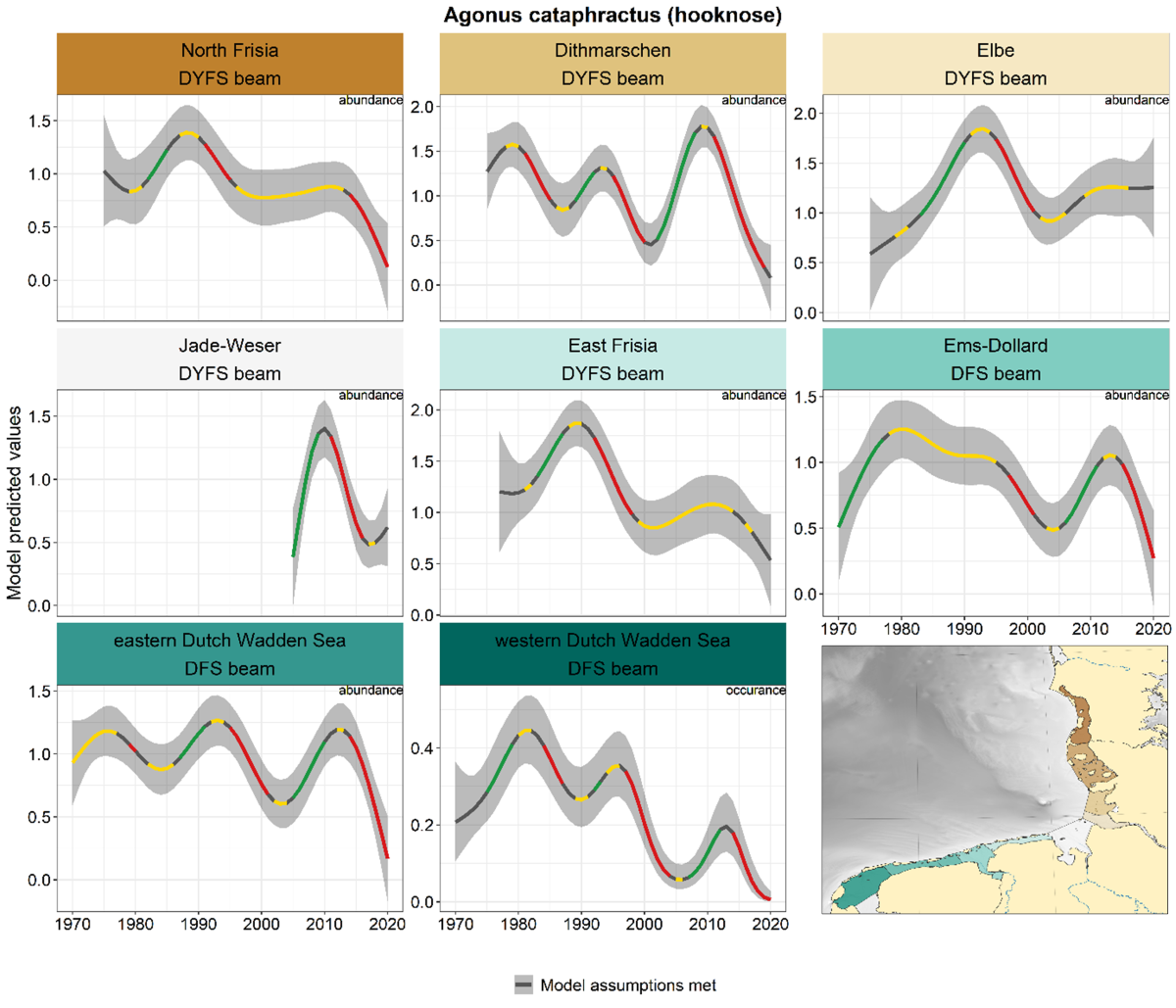Figure 18. Trends in modelled predicted abundance/probability of occurrence of hooknose in the different areas. The area-specific response variable is indicated in the top right corner of each panel. Trend lines represent GAM models. The model predicted values are on the y-axes. The grey shaded area represents the confidence interval; if the shaded area is dark grey the model assumptions are met, in the case of a light grey shaded area the model assumptions are not met. Colourcoding for the trend line: red-decrease, green-increase, yellow-stable, grey-uncertain. Because model predictions are given for a mean depth per area absolute y-values are not comparable between areas.

 

2.3.2.6 Syngnathus sp. - pipefishes

In the three most northerly areas pipefishes showed a similar development with increasing numbers from the 1980s onwards, levelling off and even declining in the past decade (Elbe, Figure 19). A strong decline after 2010 also occurred in the Jade-Weser. The development in the more southerly areas showed a different pattern, with either fluctuating trends (East Frisia, Ems-Dollard, western Dutch Wadden Sea) or a clear peak in the 1990s (eastern Dutch Wadden Sea).

 

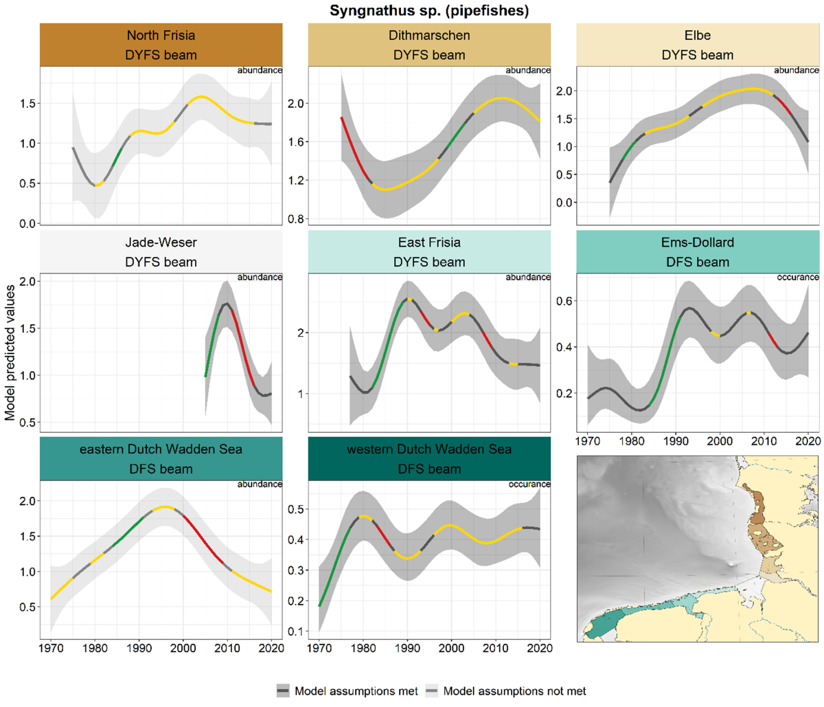Figure 19. Trends in modelled predicted abundance/probability of occurrence of pipefishes in the different areas. The area-specific response variable is indicated in the top right corner of each panel. Trend lines represent GAM models. The model predicted values are on the y-axes. The grey shaded area represents the confidence interval; if the shaded area is dark grey the model assumptions are met, in the case of a light grey shaded area the model assumptions are not met. Colour coding for the trend line: red-decrease, green-increase, yellow-stable, grey-uncertain. Because model predictions are given for a mean depth per area absolute y-values are not comparable between areas.

 

2.3.3 Diadromous species

2.3.3.1 Anguilla anguilla - eel

Eel is the only species for which we use a combination of beam trawl, stow net and fyke data. In many of the German beam trawl areas, eel is so rare that trends could not be calculated. All-time series including the 1980s showed a peak in the early 1980s (Figure 20). Several time series showed a second, lower peak around 2000. All-time series indicated very low levels of abundance or occurrence in recent times, with exception of the WMR fyke in the western Dutch Wadden Sea, showing a remarkable increase since 2010.
 
The recruitment series (glass eel and/or young yellow eel) showed general declines in the Dutch and Danish series, whereas the Danish series seems to have stabilised in the last decade (Figure 21). The German series only started in 2010 and fluctuates.

 

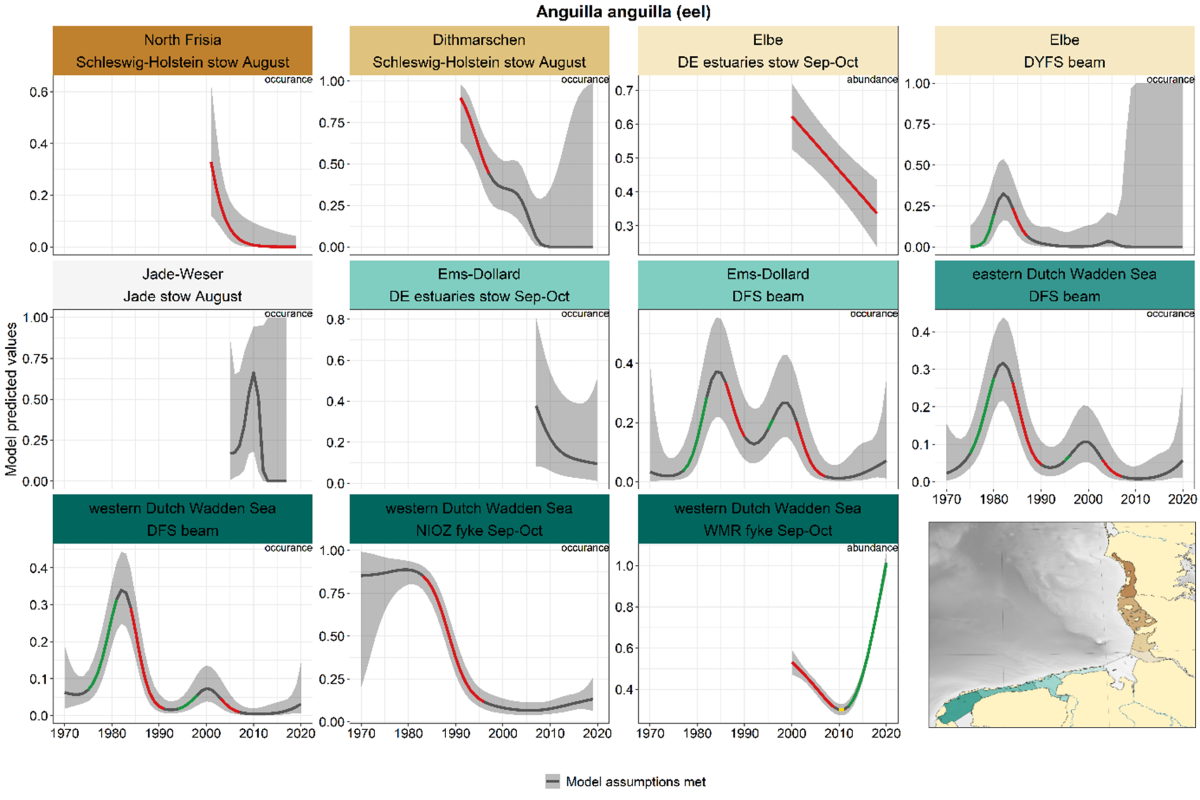Figure 20. Trends in modelled predicted abundance/probability of occurrence of eel in the different areas. The area-specific response variable is indicated in the top right corner of each panel. Trend lines represent GAM models. The model predicted values are on the y-axes. The grey shaded area represents the confidence interval; if the shaded area is dark grey the model assumptions are met, in the case of a light grey shaded area the model assumptions are not met. Colour coding for the trend line: red-decrease, green-increase, yellow-stable, grey-uncertain. Because model predictions are given for a mean depth per area absolute y-values are not comparable between areas.

 

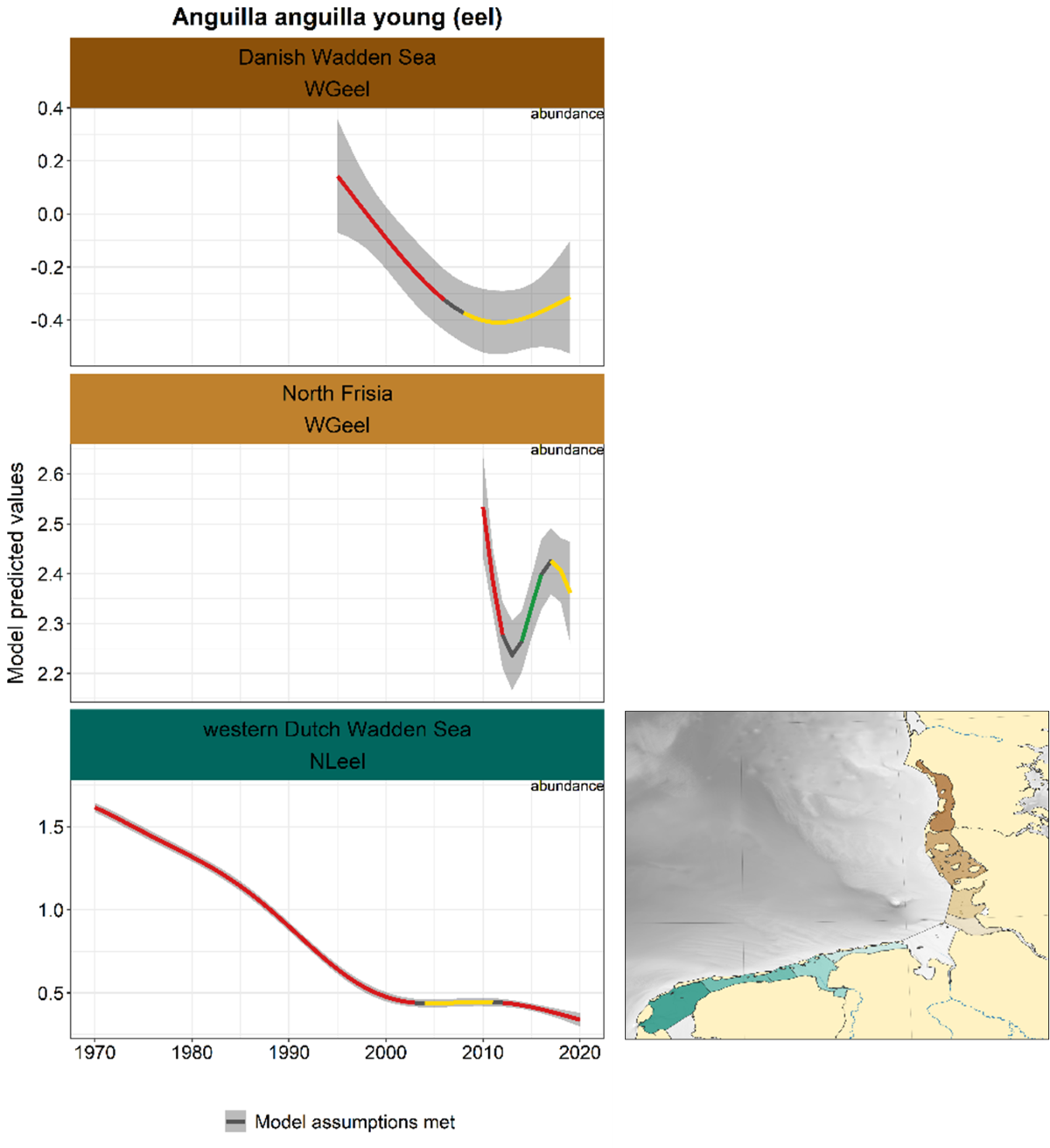Figure 21. Trends in modelled predicted abundance/probability of occurrence of young eel in the different areas. The area-specific response variable is indicated in the top right corner of each panel. Trend lines represent GAM models. The model predicted values are on the y-axes. The grey shaded area represents the confidence interval; if the shaded area is dark grey the model assumptions are met, in the case of a light grey shaded area the model assumptions are not met. Colour coding for the trend line: red-decrease, green-increase, yellow-stable, grey-uncertain. Because model predictions are given for a mean depth per area absolute y-values are not comparable between areas.

 

2.3.3.2 Osmerus eperlanus – smelt 

For smelting, the trends in spring and summer-autumn were analysed separately, because in or near the estuaries these seasons represent the spawning run (spring, adults) and the return of the juveniles (summer-autumn). This distinction between adults and juveniles by season is not possible for sampling further offshore (Jade and Schleswig-Holstein stow nets).

Spring: The time series in spring are limited in number and length, and trends vary across areas (Figure 22). In the western Dutch Wadden Sea and the Elbe, smelt numbers decrease in the last decade. A similar decrease occurred in Jade-Weser with a slightly later onset. The abundance in the Ems-Dollard was stable.

Summer-autumn: In all series apart from the Ems-Dollard recent declines occurred (although the trend is not significantly negative in North Frisia and Jade-Weser, Figure 23). Another similarity is the increase over the period 2000-2010, which is visible in Dithmarschen, Elbe and western Dutch Wadden Sea. The longest series, the NIOZ fyke, showed an uncertain trend up to the late 1990s followed by an increase and a subsequent decrease since 2013. A recent increase occurred in the Ems-Dollard. These juvenile smelts are most probably not recruits from the Ems estuary, as the structural conditions (fluid mud, oxygen deficits) of the potential spawning areas located in the Lower Ems do not allow successful reproduction. 

 

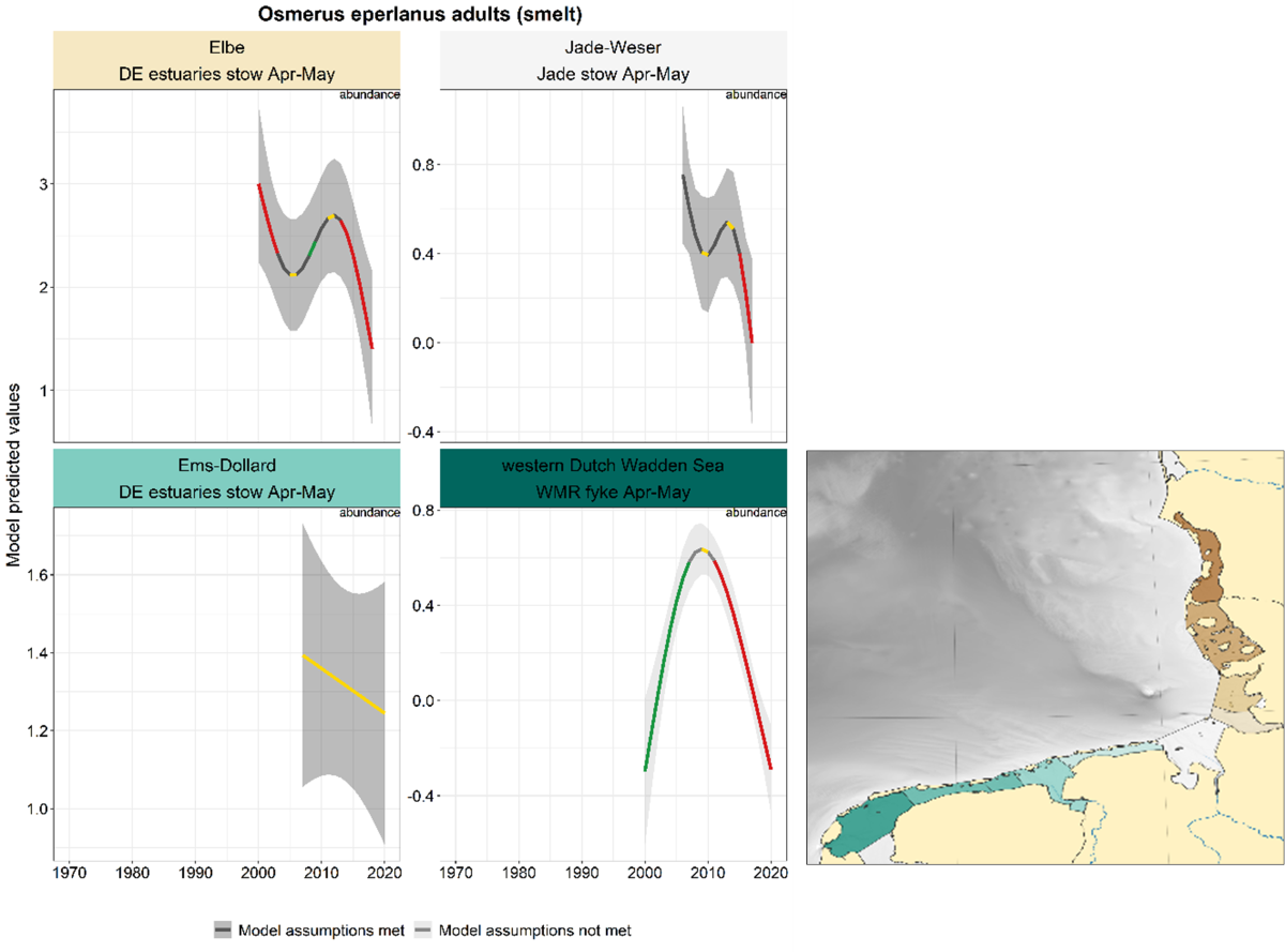Figure 22. Trends in modelled predicted abundance/probability of occurrence of adult smelt in the different areas. The area-specific response variable is indicated in the top right corner of each panel. Trend lines represent GAM models. The model predicted values are on the y-axes. The grey shaded area represents the confidence interval; if the shaded area is dark grey the model assumptions are met, in the case of a light grey shaded area the model assumptions are not met. Colour coding for the trend line: red-decrease, green-increase, yellow-stable, grey-uncertain. Because model predictions are given for a mean depth per area absolute y-values are not comparable between areas.

 

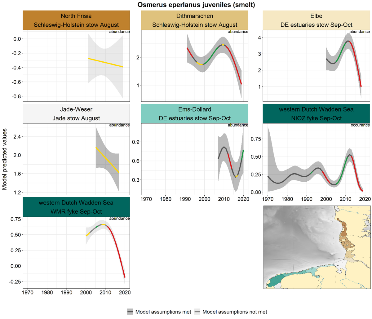Figure 23. Trends in modelled predicted abundance/probability of occurrence of juvenile smelt in the different areas. The area-specific response variable is indicated in the top right corner of each panel. Trend lines represent GAM models. The model predicted values are on the y-axes. The grey shaded area represents the confidence interval; if the shaded area is dark grey the model assumptions are met, in the case of a light grey shaded area the model assumptions are not met. Colour coding for the trend line: red-decrease, green-increase, yellow-stable, grey-uncertain. Because model predictions are given for a mean depth per area absolute y-values are not comparable between areas.

 

2.3.3.3 Alosa fallax - twaite shad

For twaite shad, like for smelt, the trends in spring (adults) and summer-autumn (juveniles) were analysed separately. Also for twaite shad, this distinction between adults and juveniles by season is not possible for sampling further offshore (Jade stow nets).

Spring: In all series except the Elbe, twaite shad decreased from 2010 onwards (but the trend is not significant in Jade-Weser and Ems-Dollard, Figure 24). The pattern in the Elbe is entirely different, with a stable trend until 2010 and a subsequent increase.

Summer-autumn:  Similar developments occur in summer-autumn, with declines from 2005-2010 onwards (not all significant, Figure 25). The only exception is again the Elbe where the trend is stable. The longest series, the NIOZ fyke, revealed a stable trend for most of the period with significant declines around the 1980s and from 2005 onwards. 

 

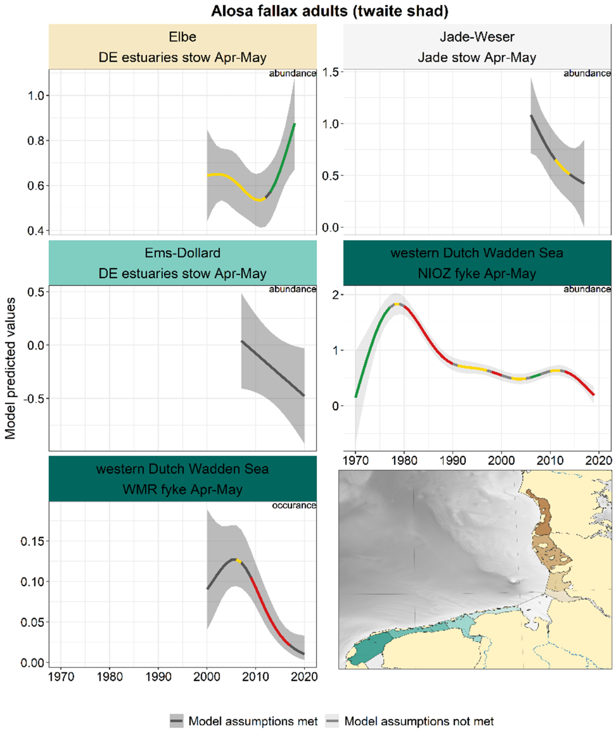Figure 24. Trends in modelled predicted abundance/probability of occurrence of adult twaite shad in the different areas. The area-specific response variable is indicated in the top right corner of each panel. Trend lines represent GAM models. The model predicted values are on the y-axes. The grey shaded area represents the confidence interval; if the shaded area is dark grey the model assumptions are met, in the case of a light grey shaded area the model assumptions are not met. Colourcoding for the trend line: red-decrease, green-increase, yellow-stable, grey-uncertain. Because model predictions are given for a mean depth per area absolute y-values are not comparable between areas.

 

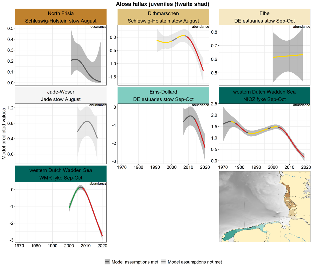Figure 25. Trends in modelled predicted abundance/probability of occurrence of juvenile twaite shad in the different areas. The area-specific response variable is indicated in the top right corner of each panel. Trend lines represent GAM models. The model predicted values are on the y-axes. The grey shaded area represents the confidence interval; if the shaded area is dark grey the model assumptions are met, in the case of a light grey shaded area the model assumptions are not met. Colourcoding for the trend line: red-decrease, green-increase, yellow-stable, grey-uncertain. Because model predictions are given for a mean depth per area absolute y-values are not comparable between areas.

 

2.3.3.4 Lampetra fluviatilis - river lamprey

Data on river lamprey is limited to only a few series because the species is quite rare. In most series (apart from the Elbe estuary) catches declined over the period 2000-2010 (Figure 26). In the Ems-Dollard and Jade-Weser numbers stabilised since. 

 

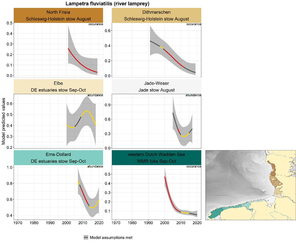Figure 26. Trends in modelled predicted abundance/probability of occurrence of river lamprey in the different areas. The area-specific response variable is indicated in the top right corner of each panel. Trend lines represent GAM models. The model predicted values are on the y-axes. The grey shaded area represents the confidence interval; if the shaded area is dark grey the model assumptions are met, in the case of a light grey shaded area the model assumptions are not met. Colour coding for the trend line: red-decrease, green-increase, yellow-stable, grey-uncertain. Because model predictions are given for a mean depth per area absolute y-values are not comparable between areas.

 

2.3.3.5 Petromyzon marinus - sea lamprey

For sea lamprey, only two trend analyses are available: from the Elbe estuary and the WMR fyke in the western Dutch Wadden Sea, since 2000 (Figure 27). The trend in the Elbe is uncertain, whereas in the western Dutch Wadden Sea the trend shows a significant and continuous decline.

 

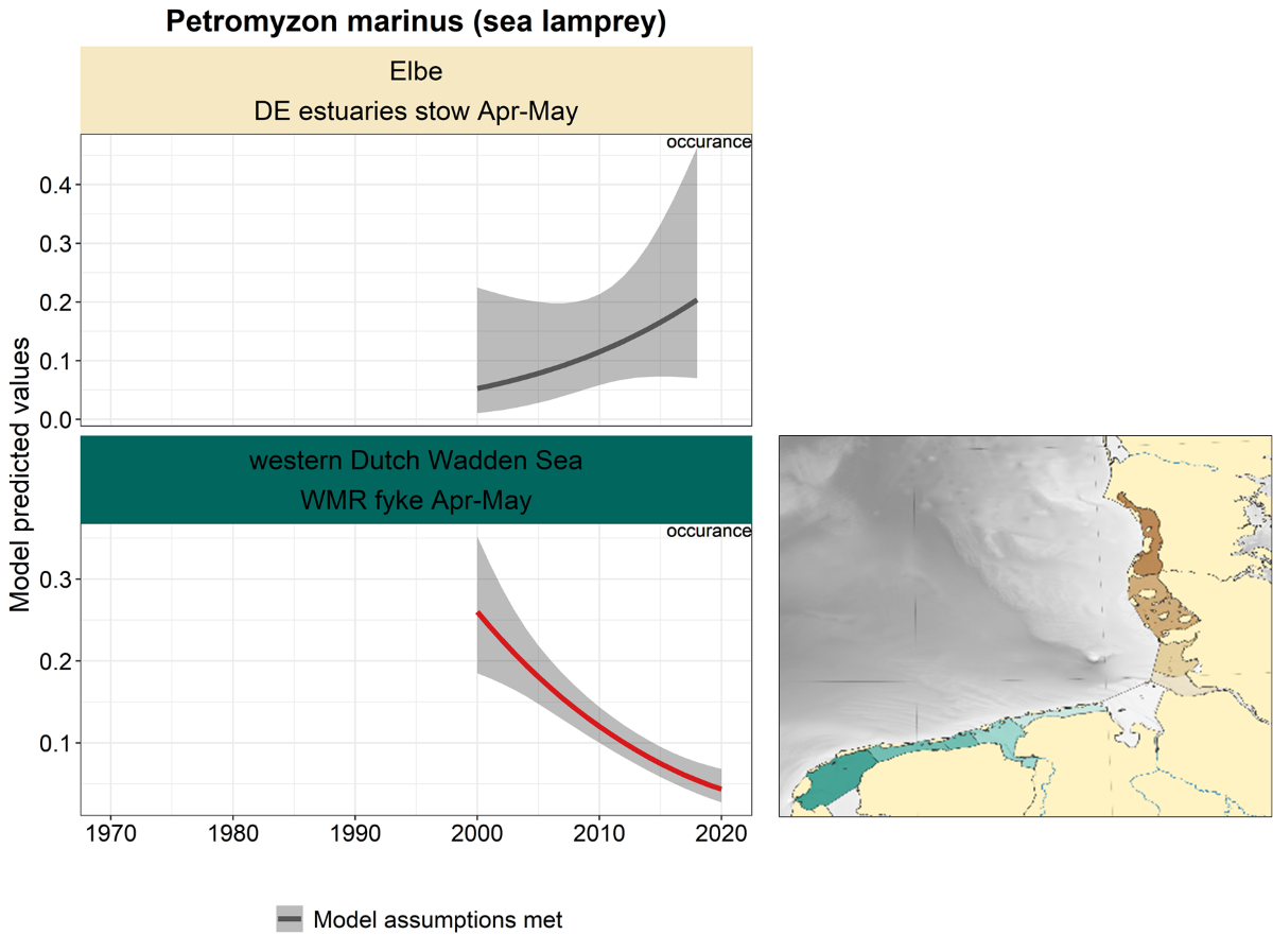Figure 27. Trends in modelled predicted abundance/probability of occurrence of sea lamprey in the different areas. The area-specific response variable is indicated in the top right corner of each panel. Trend lines represent GAM models. The model predicted values are on the y-axes. The grey shaded area represents the confidence interval; if the shaded area is dark grey the model assumptions are met, in the case of a light grey shaded area the model assumptions are not met. Colour coding for the trend line: red-decrease, green-increase, yellow-stable, grey-uncertain. Because model predictions are given for a mean depth per area absolute y-values are not comparable between areas.

 

2.3.3.6 Salmo salar – salmon

For salmon, only two surveys provided sufficient data for trend analysis (Figure 28). The trend in the Elbe is uncertain. In the Danish Wadden sea, salmon shows a sharp increase since the start of the survey, with stabilisation since roughly 2010. 

 

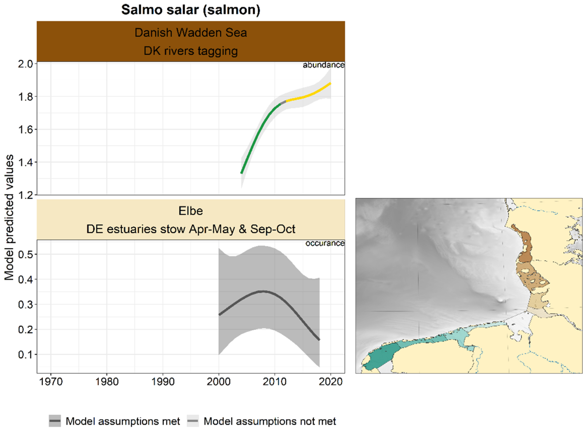Figure 28. Trends in modelled predicted abundance/probability of occurrence of salmon in the different areas. The area-specific response variable is indicated in the top right corner of each panel. Trend lines represent GAM models. The model predicted values are on the y-axes. The grey shaded area represents the confidence interval; if the shaded area is dark grey the model assumptions are met, in the case of a light grey shaded area the model assumptions are not met. Colour coding for the trend line: red-decrease, green-increase, yellow-stable, grey-uncertain. Because model predictions are given for a mean depth per area absolute y-values are not comparable between areas.

 

2.3.3.7 Salmo trutta - sea trout

Sea trout shows a stable trend in the Elbe area (Figure 29). In the western Dutch Wadden Sea, there is an increase until roughly 1983, after which the probability of occurrence showed alternating declining, stable and uncertain periods.

 

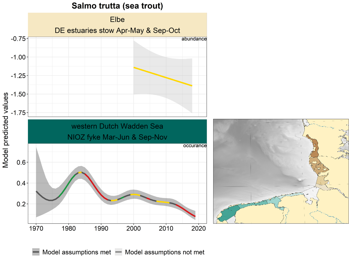Figure 29. Trends in modelled predicted abundance/probability of occurrence of sea trout in the different areas. The area-specific response variable is indicated in the top right corner of each panel. Trend lines represent GAM models. The model predicted values are on the y-axes. The grey shaded area represents the confidence interval; if the shaded area is dark grey the model assumptions are met, in the case of a light grey shaded area the model assumptions are not met. Colourcoding for the trend line: red-decrease, green-increase, yellow-stable, grey-uncertain. Because model predictions are given for a mean depth per area absolute y-values are not comparable between areas.

 

2.3.3.8 Coregonus oxyrinchus - North Sea houting 

In the Danish Wadden Sea, the North Sea houting decreased until 2000, after which the trend stabilized (Figure 30). In the western Dutch Wadden Sea, the trend fluctuates strongly, with a significant increase since 2015.
 

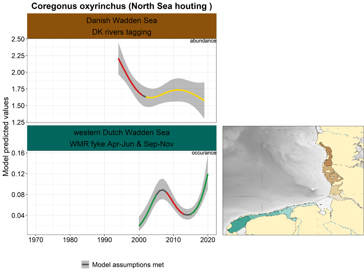Figure 30. Trends in modelled predicted abundance/probability of occurrence of North Sea houting in the different areas. The area-specific response variable is indicated in the top right corner of each panel. Trend lines represent GAM models. The model predicted values are on the y-axes. The grey shaded area represents the confidence interval; if the shaded area is dark grey the model assumptions are met, in the case of a light grey shaded area the model assumptions are not met. Colourcoding for the trend line: red-decrease, green-increase, yellow-stable, grey-uncertain. Because model predictions are given for a mean depth per area absolute y-values are not comparable between areas.

 

2.3.4 Marine adventitious and seasonal migrant species

In this group, we analysed three species that belong to the so-called small pelagics. In fact, herring also belongs to this group but has already been discussed under the marine juvenile section. Small pelagics are representatively sampled with stow nets and fykes. 

2.3.4.1 Sprattus sprattus - sprat

Trends for sprat are mainly derived from the stow net series and show large differences between the areas (Figure 31). Sprat is only occasionally caught in the NIOZ fyke; the probability of occurrence increased in the 1980s and decreased since. A decrease in abundance was observed in Dithmarschen in 1995-2010, followed by a steep increase in the last decade. The trend in the Elbe estuary is uncertain, negative in Jade-Weser and positive in the Ems-Dollard. 

 

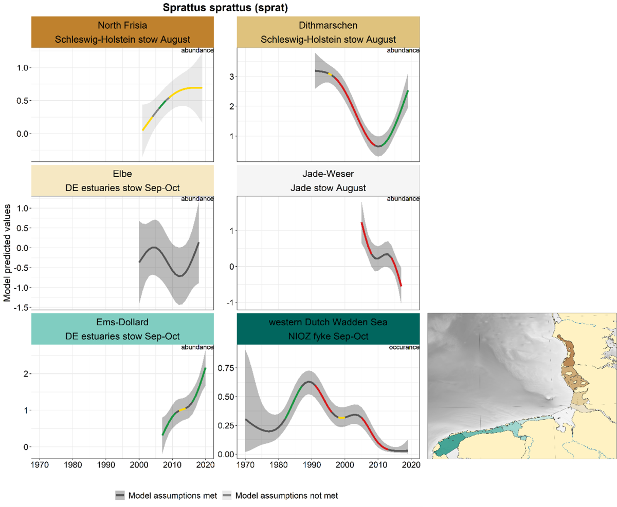Figure 31. Trends in modelled predicted abundance/probability of occurrence of sprat in the different areas. The area-specific response variable is indicated in the top right corner of each panel. Trend lines represent GAM models. The model predicted values are on the y-axes. The grey shaded area represents the confidence interval; if the shaded area is dark grey the model assumptions are met, in the case of a light grey shaded area the model assumptions are not met. Colourcoding for the trend line: red-decrease, green-increase, yellow-stable, grey-uncertain. Because model predictions are given for a mean depth per area absolute y-values are not comparable between areas.

 

2.3.4.2 Engraulis encrasicolus - anchovy

Also for anchovy, there are large differences between areas, with uncertain trends in many periods (Figure 32). Significant changes were observed in Dithmarschen and Jade-Weser (increases) and some slight decreases in the Western Dutch Wadden Sea.

 

Figure 32. Trends in modelled predicted abundance/probability of occurrence of anchovy in the different areas. The area-specific response variable is indicated in the top right corner of each panel. Trend lines represent GAM models. The model predicted values are on the y-axes. The grey shaded area represents the confidence interval; if the shaded area is dark grey the model assumptions are met, in the case of a light grey shaded area the model assumptions are not met. Colourcoding for the trend line: red-decrease, green-increase, yellow-stable, grey-uncertain. Because model predictions are given for a mean depth per area absolute y-values are not comparable between areas.

 

2.3.4.3 Sardina pilchardus - pilchard

Pilchard was only caught in the NIOZ fyke in the western Dutch Wadden Sea, but its occurrence was too rare for trend estimation. The raw data show however that this is an upcoming species, with increasing occurrence from 1995 onwards (Annex 3).

 

2.4    Species list

In the past decade (2011-2020), a total of 124 species were recorded in the long-term monitoring programmes that were used for the trend analysis (Table 3). As a result of location, period, method and total sampling effort, the total number of species per survey varied between 42 (Schleswig-Holstein stow net) and 94 (WMR fyke). The two-beam trawl surveys had a highly similar species list with few differences. The WMR fyke and German estuaries stow nets recorded most species, due to their locations, catching both marine and freshwater species.

 

Table 3. Species list by the survey for the period 2011-2020. Common names are missing for species groups that were identified to genus level only in specific programmes.

 

 

2.5    Rare species

Most of the rare species mainly occur in offshore habitats or freshwater and will occur sporadically in the Wadden Sea area. Additionally, some species that were recorded are real vagrants and probably were introduced temporarily by unusual hydrographic features (e.g. Helicolenus dactylopterus, Maurolicus muelleri).
 
The monitoring programs rarely record elasmobranch species, although some of them might use the Wadden Sea area as a nursery or as regular habitat (see section 2.6). The Jade stow net monitoring recorded all five elasmobranchs which occur in the species list.

The lesser spotted dogfish (Scyliorhinus canicula, Figure 33a) was recorded by five out of seven monitoring programs and thus seems fairly common given the assumed low catchability for elasmobranchs in the used gears. However, from the ongoing standard monitoring programs, it is not possible to derive any trends for elasmobranchs, and their abundance, distribution patterns and the possible function of the Wadden Sea as a habitat for these species remains unclear.

Several coastal monitoring programs indicate that sea horses (Hippocampus sp., Figure 33b) occur more frequently in the continental coastal waters of the North Sea in recent years. In 2020, in the coastal part of the DFS and DYFS surveys, sea horses were recorded especially along the south-westerly coasts of the Wadden Sea up to East Frisia. The causes for this increase remain unclear. It might be possible that warmer water temperatures favour a northward shift of this species or that the population as such has increased.

Sea lamprey (Petromyzon marinus) is one example of a species which is quite common in the Wadden Sea area but for which the catchability of the used gears is probably too low to be recorded regularly. While the stow and fyke net monitoring show records of this species, it was not recorded by the beam trawl surveys. This is a general phenomenon for a number of diadromous and pelagic fish species in the area.

 

 

Figure 33. Rare fish species in the Wadden Sea include elasmobranchs and sea horses: Left (A) Lesser spotted dogfish (Scyliorhinus canicula) (Photo: Oscar Bos); Right (B) Short-snouted sea horse (Hippocampus hippocampus) (Photo: Andreas Dänhardt).

 

2.6 Elasmobranchs
 
2.6.1 Introduction

Information on the occurrence and distribution of elasmobranchs (skates, rays and sharks) in the Wadden Sea is limited to historical data and anecdotal evidence (Walker, 1996; Poeisz et al., 2021). Although the area is considered to be an important (nursery) area for elasmobranch species, there is little scientific evidence to support this. In the wider North Sea, 14 skate & ray species and 12 shark species have historically been recorded (Dankers et al., 1979; De Vooys et al., 1991; Daan et al., 2005; Heessen, 2010; Walker and Kingma, 2013; Fock et al., 2014; Sguotti et al., 2016; Poiesz et al., 2021) (Table 4). Some of these also inhabit or visit the Wadden Sea, as shown in Tables 3 and 4. Within the Trilateral Swimway Programme, the elasmobranch species are seen as being characteristic of the marine adventitious species. Elasmobranchs vary in their habitat use and life history. Some are pelagic, others are demersal (Table 4).

Monitoring and research dedicated to sharks and rays in the Wadden Sea are lacking, and records are often anecdotal or originate from (historical) fisheries bycatch, surveys such as the Demersal Fish Survey (DFS) or for the North Sea from the International Bottom Trawl Survey (IBTS) (Daan et al., 2005). These surveys are not primarily designed for elasmobranchs but the data can be used to identify long-term trends (ICES 2020). Contemporary research to understand migratory patterns of shark species in the Wadden Sea area and beyond utilises satellite tags (Thorburn et al., 2019, Waddentools Swimway Waddenzee and Life-IP Deltanatuur). 

There are some (contemporary) records of sharks and rays being bycaught in shrimp fisheries in the Dutch and German Wadden Sea (P. Molenaar, R. Vorberg, pers. comm.). The MSC certified shrimp fishery is obliged to record sharks and rays in the course of their ETP-species registration program, but since they have to use sieve nets through which larger bycatch species can escape (Addison et al., 2017), the informative value is low. In practice, shark and ray species are hardly ever bycaught in the shrimp fishery.

 

Table 4. Shark and skate species (historically) recorded in the wider North Sea, and whether they have (historically) been recorded in the Wadden Sea. Deepwater species are highly unlikely to inhabit/visit the southern North Sea or the Wadden Sea. IUCN Red List status: DD = Data Deficient; LC = Least Concern; NT = Near Threatened; VU = Vulnerable; EN = Endangered; CR = Critically Endangered. IUCN information from: www.iucnredlist.org

 

Historical data from the Dutch Wadden Sea

At the beginning of the last century (1900-1920) there was a lively ray fishery in the Dutch Wadden Sea and northern Zuiderzee, targeting thornback and stingrays, caught in lobster nets, gillnets and trawls (Bergman, 1989; Walker, 1996; Heessen, 2010). The fisheries in the years 1919-1920 were especially yielding, but this was of short duration and a decline was seen in the 1930s.  Poiesz et al., (2021) analysed archival catch data (1946 - 1954) from the Royal NIOZ (Netherlands Institute for Sea, Research) of landings (mainly by local fishermen) of ray and shark species in the Dutch North Sea, including the Wadden Sea. They report eight species for the Wadden Sea area (Table 4). For the common stingray, the records in the Wadden Sea were quite high even compared to other areas. This species has been popular for its’ liver oil. It was generally thought that the demise of the thornback ray in the Wadden Sea in the 1930s and again after 1945 was due to over-fishing in the southern North Sea during these periods (Bergman, 1989). Rays were scarce from the mid-1950s onwards (Bergman, 1989; De Vooys et al., 1991). However, closing off the Zuiderzee by the Afsluitdijk in the 1930s, creating the freshwater Lake IJssel, also may have had an effect as this area was an important nursery area for the thornback rays and stingrays (Heessen, 2010). Thornback rays were also caught as bycatch in the German shrimp fisheries and between 1954 and 1960 a number of juveniles of about 20 cm were registered (Walker, 1996). There was a fishery on tope sharks in the Wadden Sea coastal area until the 1970s.

 

2.6.2    Local ecological knowledge

In 2018 a study was carried out in the Dutch Wadden Sea to map the temporal and spatial distribution of different sizes, sexes and species of sharks in the area and surrounding North Sea coast using local ecological knowledge (Noorlander et al., 2018). The aim of the project was to determine the presence of shark nurseries in the Dutch Wadden Sea, based on structured interviews with fishermen who had worked in the area for the past 30 years. The investigated species were tope, starry smooth-hound, lesser spotted dogfish and spurdog. The study shows that both adult and juvenile sharks likely inhabit (very) shallow waters in the Dutch Wadden Sea, mainly around the islands of Terschelling, Ameland and Schiermonnikoog (Noorlander et al., 2018). Specimen of early and later life stages and of each of the investigated species were encountered there during summers, but adult sharks appear to move away from the area during winter. The findings support the idea of the Dutch Wadden Sea as a shark nursery area.

Fishery-independent surveys and mark-recapture (MR) data from across the NE-Atlantic suggest the presence of different age classes of tope shark in the entire area with juveniles occurring in the Wadden Sea (Thorburn et al., 2019). Survey and MR data showed that immature tope sharks smaller than 40 cm were caught exclusively in continental shelf waters below a depth of 45 m, demonstrating a statistically significant relationship between habitat depth and total length (Figure 34).

 

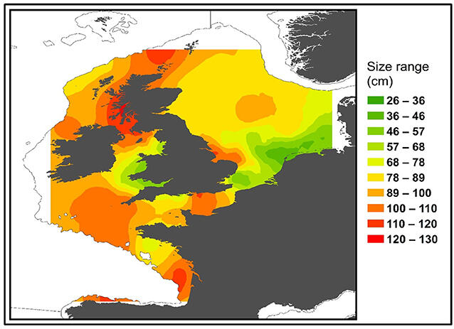Figure 34. Distribution of all immature tope sharks (Galeorhinus galeus, max length = 130 cm) based on mark and recapture and International Bottom Trawl Survey (IBTS) data sets. Colour represents the smallest sized (based on total length) animal predicted to occur in that area. From (Thorburn et al., 2019).

 

2.6.3    Historical trends in the wider North Sea

Since the Wadden Sea appears to be a nursery of shark and ray species distributed across large parts of the North Sea and the NE Atlantic, it is possible that larger-scale abundance trends are also evident in the Wadden Sea. Because Wadden Sea data are lacking we, therefore, describe the developments of several species in the wider North Sea.
 
Trends of elasmobranchs in the wider North Sea based on fishery-independent surveys have shown different patterns over the past decades (Fock et al., 2014; Sguotti et al., 2016; ICES, 2020). Whereas previous analyses of fishery-independent data from 1902 to 2013 demonstrated that larger species such as thornback ray, tope shark, and spiny dogfish showed long term declines in the southern North Sea region, more recent data have shown an increase in the thornback ray in the past 10 years. The common skate complex and angel shark were considered extinct altogether (Walker and Hislop, 1998; Nieto et al., 2015; Bom et al., 2019), but recent analyses show a small but consistent increase in the common skate complex in the past 10 years (ICES, 2020). Smaller species, such as spotted ray, starry ray, and lesser spotted dogfish but also the starry smooth-hound seem to have increased over the past decades (1902–2013) (Sguotti et al., 2016). However, since the early 2000s, the starry ray declined quite rapidly and is now on the EU prohibited species list (ICES, 2020). Fock et al. (2014) compared data from 1902-1932 with 1991 - 2009, and conclude similar results for all species except for the smooth-hound – they report a decrease in this species. When looking at a shorter time period, Daan et al. (2005) analysed the North Sea, Skagerrak and Kattegat survey data and reported a decrease in spiny dogfish and common skate, and an increase of lesser spotted dogfish, tope shark and smooth-hounds over the period 1970 – 2004. For other ray species, the trends were less clear. Recent research demonstrated that populations of thornback ray, spotted ray and blonde ray (Figure 35) all have been increasing in the North Sea area since 1990, albeit at different rates (Amelot et al., 2021).

The relationship between the abundance and distribution of skates, rays and sharks in the North Sea and those occurring in the Wadden Sea, and vice versa, is unknown. It is likely that the Wadden Sea plays a role in the life-cycle of at least some of the species, but this has never been quantified. Dedicated research is necessary to understand the population dynamics of elasmobranch species in the Wadden Sea. Hopefully, the new research projects on the migratory sharks in the Wadden Sea will hopefully provide some information.

 

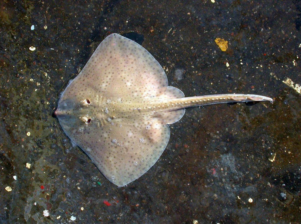Figure 35. Blonde ray (Raja brachyura) (Photo: Niels Daan).

 

3. Assessment

3.1 Trilateral targets

In their declaration from the 13th governmental council meeting in May 2018 in Leeuwarden, the trilateral ministers placed a mandate to implement the trilateral fish targets contained in the Wadden Sea Plan (CWSS, 2010):

• Viable stocks of populations and natural reproduction of typical Wadden Sea fish species.
• Occurrence and abundance of fish species according to the natural dynamics in (a)biotic conditions.
• Favourable living conditions for endangered fish species.
• Maintenance of the diversity of natural habitats to provide substratum for spawning and nursery functions for juvenile fish.
• Maintaining and restoring the possibilities for the passage of migrating fish between the Wadden Sea and inland waters

In the previous trilateral Quality Status Report, the authors of the fish thematic report noted: “These targets were not formulated in a testable way, which makes it impossible to evaluate them quantitatively. Furthermore, the formulations are not all easy to comprehend, allowing multiple interpretations.“ (Tulp et al., 2017). They, therefore, reformulated the generic targets and suggested that the next step should be the formulation of quantitative and testable sub-targets, which ”should focus on fish parameters that are influenced by (manageable) human activities“ (Tulp et al., 2017). They also pointed out that the formulation of such quantitative targets is hampered by the limited knowledge of human impacts, population dynamics and ecology of typical Wadden Sea fish species. 

The reformulated targets in 2017 are:

Overall target: There should be no human-induced bottlenecks in the Wadden Sea for fish populations or their ecosystem functions. 

Targets (all in reference to the overall target): maintain or improve:

• robust and viable populations of estuarine resident fish species.
• the nursery function of the Wadden Sea and estuaries.
• the quality and quantity of typical Wadden Sea habitats.
• passageways for fish migrating between the Wadden Sea and inland waters.

 

3.2 Trend summary and target evaluation

The generic targets can only partly, and only qualitatively be evaluated based on the trend analyses. In most cases, causes for observed trends are not known. To provide a concise overview of long term changes we summarize the trends by decade and across geographic regions (Table 5). Note that this aggregation results in a loss of detail potentially relevant for correct interpretation. Therefore it is advised to view Table 5 in conjunction with the detailed trend figures and descriptions. A comparison of overall trends with previous QSR reports, as done in other QSR thematic reports, is not feasible for fish, due to changes in methodology and species selections.

The abundance of estuarine residents varies between species and areas. In the last decade, abundance is stable for most species, except for bull-rout (Figure 36) and hooknose, which showed a decline in both the Dutch and German Wadden Sea. Whether or not populations have declined below robust and viable levels is unknown.  

In general, trends in marine juveniles are similar between the Dutch and German Wadden Sea and the strongest changes occurred in the period before 2000. Most marine juveniles have stabilised in the last decade, except sea bass (NL) and cod (DE) showing a decline, and whiting showing an increase (DE). Overall, the nursery function of the Wadden Sea appears to have declined since the 1980s and has stabilised in the last decade.
 
Based on our current analyses the target quality and quantity of typical Wadden Sea habitats cannot be evaluated.
  
For diadromous species in the Dutch Wadden Sea during the last decade, decreasing trends greatly outnumber increasing or stable trends. This is despite the fact that numerous barriers for diadromous fish in Dutch rivers have been mitigated using fish ladders. Currently, the “fish migration river” is being installed in the Dutch Afsluitdijk, which will create a passageway between the Dutch Wadden Sea and the freshwater Lake IJssel. In the German Wadden Sea, mostly stable or uncertain trends are observed in the last decade. Trends in the Danish rivers have stabilised in the last decade, for the three species examined (salmon, houting, and eel). During the last two decades, numerous river restoration projects have been carried out in the Danish rivers, improving salmonid habitat and opening up extensive new areas, thus greatly improving the production of wild salmonid juveniles. Most salmon rivers now have only very minor obstacles left. The current stabilisation of the salmon, sea trout and houting populations is likely caused by increased in-river predation from cormorants, inducing a five-fold increase in juvenile winter mortality.

The endangered fish species in the Wadden Sea are (according to Danish, German and Dutch red lists): river lamprey, sea lamprey, twaite shad, European eel, North Sea Houting, Atlantic salmon, sea stickleback, greater pipefish, snack pipefish, greater weever, poor cod, transparent goby, picked dogfish, tope shark, starry smooth-hound, common stingray and thornback ray (Thiel et al., 2013), (https://minez.nederlandsesoorten.nl/content/rode-lijsten, https://mst.dk/natur-vand/natur/national-naturbeskyttelse/naturpleje/naturplejeguiden/roedlistede-arter/). Our trend analyses only included the first six (diadromous) species and Syngnathus sp. (lesser and greater pipefish combined). Of these, only North Sea houting showed an increase, and all other species-region combinations showed declining, stable or uncertain trends.

 

Table 5. Summary of trends (all gears combined) per decade and region. The trend estimate (increase, decrease, stable or uncertain (0)) was derived by taking the mode of the estimates by year and area. The Ems stow net data were incorporated in the Dutch Wadden Sea and the Elbe stow net data in the German Wadden Sea.

 

3.3 Trilateral targets: progress and future steps

Since the previous QSR, the focus on fish in the Wadden Sea has largely increased as evidenced by the Swimway action programme, the establishment of a Swimway Working Group within the Trilateral Monitoring and Assessment Programme (TMAP), and the initiation of several research programmes.

At an international conference (SWIMWAYs: Understanding connectivity within the life cycles of coastal fish, Dänhardt, 2019), the trilateral fish targets were discussed. Here suggestions on methods, variables and indicators to progress towards testable fish targets were discussed. 

Testable targets are not only a prerequisite for scientific evaluation within the QSR framework, they are also necessary for the implementation of environmental quality objectives set by other directives. The major current conservation legislation (EU Directives Habitat, Water Framework Directive and Marine Strategy Framework) requires testable targets, and failure to reach them is threatened by monetary penalties for the member states. The generic targets need to be translated into biologically relevant and measurable indicators suitable for statistical analysis, thus forming the backbone for target specification and evaluation, and for providing the evidence base to assess the effectiveness of conservation measures.

Practically, however, it depends on the properties of the ecosystem, of the fish community and data availability, to what degree target specification is possible and makes sense. Because of the complexity and multi causality within the ecosystem and the uncertainty of the precision of fish sampling methods it is unlikely that gradual changes would immediately be visible in monitoring results. Despite these difficulties, using approximations of population size and the extent and distribution of stressors may be a feasible approach to evaluate progress toward the fish targets and the effect of possible conservation measures. Although currently still unavailable, reference to a historical state of the fish community (during times of lower levels of human activity) would allow inferences about whether the observed changes move towards or away from this reference. Whether establishing such historical references would be feasible is not known but would be worth the effort. Furthermore, changes in community metrics such as the share of rare/common species may also yield useful indications for target evaluation. 

Table 6 provides suggestions on how to proceed concerning the trilateral fish targets. A full account of future steps is far beyond the scope of this report, as this will require dedicated effort from experts.

 

Figure 36. Bull-rout (Myoxocephalus scorpius) Photo: (Oscar Bos)

 

Table 6. Trilateral fish targets (Wadden Sea Plan 2010 and revised generic targets 2017): Overview of possible research questions and indicators, and data or information required and available.  

 

4. Recommendations

4.1 Evaluation of 2017 recommendations

In 2017 a set of recommendations both for management and monitoring and research was formulated (Tulp et al., 2017). In Annex 4, these are evaluated. Below we formulate newly emerging recommendations for the period until the next evaluation.

 

4.2 Recommendations for management

Since the last QSR thematic report on fish was published in 2017, the SWIMWAY vision along with a comprehensive working programme has been launched to implement the trilateral fish targets. A trilateral SWIMWAY working group has been installed and has tackled several aspects. During a scientific conference held in September 2019 in Hamburg, all aspects relating to the trilateral fish targets have been addressed by a variety of oral and poster presentations, interactive breakout sessions and discussions in between (see conference report, Dänhardt, 2019). We recommend using the outcome of these initiatives for future steps to arrive at specific targets. We recommend that the trilateral SWIMWAY working group takes the lead in this process and takes into account the suggestions presented in Table 6. 

 

4.3 Recommendations for science and monitoring

A crucial knowledge gap hampering implementation of the trilateral fish targets is knowledge of specific bottlenecks. Bottlenecks can be defined as critical pressures that inhibit the completion of fish life cycles or inhibit the ecosystem function of fish in the Wadden Sea. Bottlenecks need to be identified, understood and, if of anthropogenic origin, removed. We still lack basic knowledge of historic references, structure and functioning of the Wadden Sea system for fish (paragraph 3). Also, mechanisms that drive developments in Wadden Sea fish stocks are not understood well enough. Such knowledge is a prerequisite for formulating testable targets for Wadden Sea fish and for being able to consider shifting/moving baselines in setting targets and goals. Since the 2017 QSR, there have been several successful initiatives to enhance knowledge of fish in the Wadden Sea. In the Netherlands, the Waddentool-Swimway program is running from 2020-2024 as a cooperative project of institutes, universities and NGOs with five PhDs and one postdoc working on different aspects (small pelagic fish, the function of saltmarshes and shellfish beds for fish, climate effects, large fish species).

Regarding scientific questions, there are still some important matters that are not covered by any of the running programs, but that need attention in order to improve the understanding of the Wadden Sea function for fish. We recommend research attention be directed at the following subjects:

1. Monitoring of underrepresented groups: pelagic fish, larger fish species, fish in specific habitats.
2. Historic situation: our regular observations of Wadden Sea fish do not go back further than the 1970s. However, there is still a lot of unexplored historical data dating further back. To understand developments on a longer time scale, we need to disclose the historic information. See for example Bom et al. (2020).
3. Relationship Wadden Sea-North Sea: what is the contribution of the Wadden Sea as a nursery area to North Sea stocks?
4. The effect of noise pollution on habitat use in the Wadden Sea. The (recreational) use of the Wadden Sea is increasing with more and more boat traffic going to and from the islands. Fishermen think this might be an important source of the disturbance.
5. The effect of different sources of mortality (predation, fisheries) on Wadden Sea fish. Are fish regulated bottom-up or top-down?
6. How did phenological changes influence the functioning of the Wadden Sea for fish (due to climate change)? Climate change may have affected arrival or emigration dates from the Wadden Sea and therefore also species interactions (e.g. predation) potentially leading to mismatches. Phenological research is a large research field in the terrestrial world, but far less in the marine world where it is probably equally important.
7. Other direct and indirect effects of climate change: are sea-level rise, change in abiotic conditions and predator-prey relationships.
8. Effects of sand nourishments: there are continuous nourishments on the North Sea shore of islands and in the tidal outlets.

 

5. Summary

The status and trends of Wadden Sea fish were based on ten different monitoring programmes that were conducted for at least ten years. In the past decade, a total of 124 different species were recorded.

We report on the developments of 25 common to fairly rare fish species belonging to different guilds in 9 subareas in the international Wadden Sea. Analysed species belong to marine juveniles (8 species), estuarine residents (6), diadromous (8), marine adventitious (1) and marine seasonal migrants (2). In addition, we provide anecdotical information on the status of sharks, skates and rays. Only species-area combinations that had a minimum of 5 % non-zero recordings were included in the formal trend analyses.

Trends in abundance of Wadden Sea fish varied between ecological guilds. After an initial increase from 1970 to 1980, fish using the Wadden Sea as a nursery area declined in nearly all subareas since the early or mid-1980s, followed by a subsequent stabilisation at a low level in the one to two most recent decades. The exception to this pattern is the Elbe. 

The nursery function of the Wadden Sea has especially changed for the traditional flatfish species such as plaice, dab and sole. Most of these declined from the 1980s onwards and levelled off until current times. Although not significant, plaice trends seemed to make an upward bend in the German areas in the past five years, while dab showed this in the Dutch areas. Sole showed a similar pattern, but while levels have stayed low in the German areas, numbers have increased in the Dutch areas after the absolute low in the 1990s. For the gadoids:  cod in all areas and whiting in Dutch areas showed a similar pattern compared to the flatfishes, with a peak in the 1980s followed by an overall decline. Whiting showed more variable patterns in German areas, with recent increases from East Frisia northwards. The increase in one of the newcomers to this guild: tub gurnard, a southern species, has levelled off or even decreased since the previous report. For the other newcomer, sea bass, the increase from the 1980s to 2000 has come to a halt or even a recent decrease.
 
For other migratory species and resident species, trends varied considerably between species, regions and time periods. Among the resident species, there were species with overall stable trends (flounder), species with an ongoing decline (eelpout and hooknose), species with variable trends (bull-rout and pipefishes) and species with an overall increase (five-bearded rockling). Amongst the diadromous species, there were generally more species-area combinations with decreasing than increasing trends. The most noteworthy trends were the increase of salmon and decrease of North Sea houting in Danish Wadden Sea rivers and the overall decrease of eel in all areas and gears.

Despite the fact that the Wadden Sea may be an important (nursery) area for elasmobranch species (skates and sharks), information on their spatial and temporal occurrence and distribution in the Wadden Sea are scarce because the standard monitoring programs are unsuitable to catch these species. For several species occurring in the North Sea, it is likely that they also inhabit or visit the Wadden Sea, and for some (e.g. tope shark, lesser spotted dogfish) there have indeed been observations within the Wadden Sea. In the wider North Sea region, many elasmobranch species have strongly declined and/or are considered (near-) extinct.

As the trilateral fish targets are described in an abstract manner, they cannot be evaluated quantitatively. Therefore we evaluated the targets in a qualitative manner only.

The abundance of estuarine residents in the last decade abundance is stable for most species, except for bull-rout and hooknose, who showed a decline in both the Dutch and German Wadden Sea. In general, trends in marine juveniles are similar between the Dutch and German Wadden Sea and the strongest changes occurred in the period before 2000. Most marine juveniles have stabilised in the last decade.  Overall, the nursery function of the Wadden Sea appears to have declined since the 1980s and has stabilised in the last decade. Based on our current analyses the target quality and quantity of typical Wadden Sea habitats cannot be evaluated. Amongst the diadromous species, decreasing species greatly outnumber increasing species in the last decade. Trends in the Danish rivers have stabilised for all three species (salmon, houting and eel) in the last decade. The endangered fish species included in the trend analyses (mainly diadromous species) show decreasing, stable or uncertain trends in the last decade, except North Sea houting, which shows an increase in the Dutch Wadden Sea.
 
We conclude with a sketch of how progress towards more testable targets can be achieved and provide recommendations for future research.

 

About the authors I. Tulp1, L. Bolle2, Chun Chen1, A. Dänhardt3, H. Haslob4, N. Jepsen5, A. van Leeuwen6, S. Poiesz1, J. Scholle7, J. Vrooman1, R. Vorberg8, P. Walker9   1 Wageningen Marine Research, IJmuiden, NL 2 Nouvelle-Aquitaine Eco Studies, Saint-Moreil, FR 3 Independent researcher, Jesteburg / Lüllau, DE 4 Thünen Institute of Sea Fisheries, Braunschweig, DE 5 DTU AQUA, Kgs. Lyngby, DK 6 Netherlands Institute for Sea Research, 't Horntje (Texel), NL 7 BIOCONSULT Schuchardt & Scholle GbR, Bremen, DE 8 Marine Science Service, Dassendorf, DE 9 Tethys: aquatic ecosystem advice, Engwierum, NL

References

Addison, J., G. Gaudian, and P. Knapman. 2017. MSC Sustainbale Fisheries Certification. North Sea Brown Shrimp. Public Certification Report. Acoura Marine Ltd.
Alheit, J., T. Pohlmann, M. Casini, W. Greve, R. Hinrichs, M. Mathis, K. O'Driscoll, R. Vorberg, and C. Wagner. 2012. Climate variability drives anchovies and sardines into the North and Baltic Seas. Progress in Oceanography 96:128-139.
Amelot, M., J. Batsleer, E. Foucher, R. Girardin, P. Marchal, J. J. Poos, and K. Sys. 2021. Evidence of difference in landings and discards patterns in the English Channel and North Sea Rajidae complex fishery. Fisheries Research 242:106028.
Bergman, M. J. N. 1989. De rog (Raja davata, Raja batis, Dasyatis pastinaca). Page 14 Ecologisch Profiel Vissen, Literature study. Rijkswaterstaat, Dienst Getijdewateren.
Bolle, L. J., T. Neudecker, R. Vorberg, U. Damm, B. Diederichs, J. Scholle, Z. Jager, A. Dänhardt, G. Lüerßen, and H. Marencic. 2009. Trends in Wadden Sea fish fauna. C108/08, Wageningen IMARES Report
Bom, R. A., M. van de Water, A. Brader, H. W. van der Veer, and A. van Leeuwen. 2019. The historical occurrence of the angelshark Squatina squatina and common skate Dipturus batis in Dutch coastal waters. NIOZ-report.
Bom, R. A., M. van de Water, K. C. J. Camphuysen, H. W. van der Veer, and A. van Leeuwen. 2020. The historical ecology and demise of the iconic Angelshark Squatina squatina in the southern North Sea. Marine Biology 167:91.
CWSS. 2010. Wadden Sea Plan. 11th Trilateral Governmental Conference on the Protection of the Wadden Sea, Westerland/Sylt 18 March 2010. Common Wadden Sea Secretariat (CWSS), Wilhelmshaven, Germany.
Daan, N., H. Heessen, and R. ter Hofstede. 2005. North Sea Elasmobranchs: distribution, abundance and biodiversity. ICES.
Dänhardt, A. 2019. SWIMWAYs: Understanding connectivity within the life cycles of coastal fish. Conference report, 24-26 September 2019, Hamburg, Germany. Jesteburg/ Lüllau, 105 pages. Common Wadden Sea Secretariat, Wilhelmshaven, Germany.
Dänhardt, A., and P. H. Becker. 2011. Does small-scale vertical distribution of juvenile schooling fish affect prey availability to surface-feeding seabirds in the Wadden Sea? Journal of Sea Research 65:247-255.
Dankers, N., W. J. Wolff, and J. J. Zijlstra. 1979. Fishes and fisheries of the Wadden Sea. AA Balkema.
De Vooys, C., J. Witte, R. Dapper, J. Van der Meer, and H. Van der Veer. 1991. Lange termijn veranderingen in zeldzame vissoorten op het Nederlands continentaal plat van de Noordzee. http://www.vliz.be/imisdocs/publications/61/313761.pdf.
Elliott, M., and K. Hemingway. 2002. Fishes in estuaries. Blackwell Science.
Elliott, M., A. K. Whitfield, I. C. Potter, S. J. M. Blaber, D. P. Cyrus, F. G. Nordlie, and T. D. Harrison. 2007. The guild approach to categorizing estuarine fish assemblages: a global review. Fish and Fisheries 8:241-268.
Fock, H. O., W. N. Probst, and M. Schaber. 2014. Patterns of extirpation. II. The role of connectivity in the decline and recovery of elasmobranch populations in the German Bight as inferred from survey data. Endangered Species Research 25:209-223.
Heessen, H. J. L. 2010. State of the Art-Haaien en roggen in de Noordzee. IMARES.
ICES. 2020. Working Group on Elasmobranch Fishes (WGEF). International Council for the Exploration of the Sea.
Nieto, A., Ralph, G.M., Comeros-Raynal, M.T., Kemp, J., García Criado, M., Allen, D.J.,, N. K. Dulvy, Walls, R.H.L., Russell, B., Pollard, D., García, S., Craig, M., Collette, B.B.,, R. Pollom, Biscoito, M., Labbish Chao, N., Abella, A., Afonso, P., Álvarez, H., Carpenter, K.E.,, S. Clò, Cook, R., Costa, M.J., Delgado, J., Dureuil, M., Ellis, J.R., Farrell, E.D., Fernandes, P., A.-B. Florin, Fordham, S., Fowler, S., Gil de Sola, L., Gil Herrera, J., Goodpaster, A., Harvey,, H. M., H., Herler, J., Jung, A., Karmovskaya, E., Keskin, C., Knudsen, S.W., Kobyliansky,, K. S., M., Lawson, J.M., Lorance, P., McCully Phillips, S., Munroe, T., Nedreaas,, N. K., J., Papaconstantinou, C., Polidoro, B., Pollock, C.M., Rijnsdorp, A.D., Sayer, C.,, and J. Scott, Serena, F., Smith-Vaniz, W.F., Soldo, A., Stump, E. and Williams, J.T,. 2015. European Red List of marine fishes. 9279454129, Publications Office of the European Union, Luxembourgh.
Noorlander, K., S. Maycock, and P. A. Walker. 2018. Local ecological knowledge on spatial and temporal distribution of sharks in the Dutch Wadden Sea and North Sea. VHL/NEV/Aeres.
Poiesz, S. S. H., T. van Elderen, J. I. Witte, and H. W. van der Veer. 2021. Historical trophic ecology of some divergent shark and skate species in the Dutch coastal North Sea zone. Marine Biology, 168(11):1-15.
Sguotti, C., C. P. Lynam, B. García‐Carreras, J. R. Ellis, and G. H. Engelhard. 2016. Distribution of skates and sharks in the North Sea: 112 years of change. Global change biology 22:2729-2743.
Thiel, R., H. Winkler, U. Böttcher, A. Dänhardt, R. Fricke, M. George, M. Kloppmann, T. Schaarschmidt, C. Ubl, and R. Vorberg. 2013. Rote Liste und Gesamtartenliste der etablierten Fische und Neunaugen (Elasmobranchii, Actinopterygii & Petromyzontida) der marinen Gewässer Deutschlands. In: Becker, N.; Haupt, H.; Hofbauer, N.; Ludwig, G. & Nehring, S. (Red.): Rote Liste gefährdeter Tiere, Pflanzen und Pilze Deutschlands, Band 2: Meeresorganismen. – Münster (Landwirtschaftsverlag). – Naturschutz und Biologische Vielfalt 70 (2):11-76.
Thorburn, J., F. Neat, I. Burrett, L.-A. Henry, D. M. Bailey, C. S. Jones, and L. R. Noble. 2019. Ontogenetic variation in movements and depth use, and evidence of partial migration in a benthopelagic elasmobranch. Frontiers in Ecology and Evolution 7:353.
Tulp I., Bolle L.J., Dänhardt A., de Vries P., Haslob H., Jepsen N., Scholle J. & van der Veer H.W. 2017. Fish. In: Wadden Sea Quality Status Report. Eds.: Kloepper S. et al., Common Wadden Sea Secretariat, Wilhelmshaven, Germany. Last updated 21.12.2017. qsr.waddensea-worldheritage.org/reports/fish-2017
van der Veer, H. W., R. Berghahn, J. M. Miller, and A. D. Rijnsdorp. 2000. Recruitment in flatfish, with special emphasis on North Atlantic species: Progress made by the Flatfish Symposia. Ices Journal of Marine Science 57:202-215.
Visser, H. 2004. Estimation and detection of flexible trends. Atmospheric Environment 38:4135-4145.
Walker, P. 1996. Ecoprofile rays and skates on the Dutch continental shelf and North Sea.
Walker, P., and I. Kingma. 2013. Onderzoek naar haaien en roggen in Nederland in het kader van de Kaderrichtlijn Mariene Strategie. Eindrapportage Fase 1., Nederlandse Elasmobranchen Vereniging, Amsterdam.
Walker, P. A., and J. R. G. Hislop. 1998. Sensitive skates or resilient rays? Spatial and temporal shifts in ray species composition in the central and north-western North Sea between 1930 and the present day. ICES Journal of Marine Science 55:392-402.
Witte, J. Y., and J. J. Zijlstra. 1978. the species of fish occurring in the Wadden Sea.in N. Dankers, W. J. Wolff, and J. J. Zijlstra, editors. Fishes and fisheries of the Wadden Sea. Stichting Veth tot Steun aan Waddenonderzoek, Leiden.
This report should be cited as: Tulp, I., Bolle, L. J., Chen, C., Dänhardt, A., Haslob, H., Jespen, N., van Leeuwen, A., Poiesz, S., Scholle, J., Vrooman, J., Vorberg, R., & Walker, P. (2022). Wadden Sea Quality Status Report: Fish. Common Wadden Sea Secretariat. https://doi.org/10.5281/zenodo.15223705
All 2022 reports may be cited collectively as: Kloepper, S., Bostelmann, A., Bregnballe, T., Busch, J.A., Buschbaum, C., Deen, K., Domnick, A., Gutow, L., Jensen, K., Jepsen, N., Luna, S., Meise, K., Teilmann, J., & van Wezel, A. (2022). Wadden Sea Quality Status Report. Common Wadden Sea Secretariat, Wilhelmshaven, Germany. Downloaded DD.MM.YYYY. qsr.waddensea-worldheritage.org